Outlier detection with FPCA

Example of using the inverse_transform method in the FPCA class to detect outlier(s) from the reconstruction (truncation) error.

In this example, we illustrate the utility of the inverse_transform method of the FPCA class to perform functional outlier detection. Roughly speaking, an outlier is a sample which is not representative of the dataset or different enough compared to a large part of the dataset. The intuition is the following: if the eigenbasis, i.e. the q>=1 first functional principal components (FPCs), is sufficient to linearly approximate a clean set of samples, then the error between an observed sample and its approximation w.r.t to the first ‘q’ FPCs should be small. Thus a sample with a high reconstruction error (RE) is likely an outlier, in the sense that it is underlied by a different covariance function compared the training samples (nonoutliers).

# Author: Clément Lejeune
# License: MIT

import matplotlib.pyplot as plt
import numpy as np
from scipy.stats import gaussian_kde

from skfda.datasets import make_gaussian_process
from skfda.misc.covariances import Exponential, Gaussian
from skfda.misc.metrics import l2_distance, l2_norm
from skfda.preprocessing.dim_reduction import FPCA

We proceed as follows: - We generate a clean training dataset (not supposed to contain outliers) and fit an FPCA with ‘q’ components on it. - We also generate a test set containing both nonoutliers and outliers samples. - Then, we fit an FPCA(n_components=q) and compute the principal components scores of train and test samples. - We project back the principal components scores, with the inverse_transform method, to the input (training data space). This step can be seen as the reverse projection from the eigenspace, spanned by the first FPCs, to the input (functional) space. - Finally, we compute the relative L2-norm error between the observed functions and their FPCs approximation. We flag as outlier the samples with a reconstruction error (RE) higher than a quantile-based threshold. Hence, an outlier is thus a sample that exhibits a different covariance function w.r.t the training samples.

The train set is generated according to a Gaussian process with a Gaussian (i.e. squared-exponential) covariance function.

grid_size = 100

cov_clean = Gaussian(variance=2.0, length_scale=5.0)

n_train = 10**3
train_set = make_gaussian_process(
    n_samples=n_train,
    n_features=grid_size,
    start=0.0,
    stop=25.0,
    cov=cov_clean,
    random_state=20
)
train_set_labels = np.array(['train(nonoutliers)'] * n_train)

The test set is generated according to a Gaussian process with the same covariance function for nonoutliers (50%) and with an exponential covariance function for outliers (50%).

n_test = 50
test_set_clean = make_gaussian_process(
    n_samples=n_test // 2,
    n_features=grid_size,
    start=0.0,
    stop=25.0,
    cov=cov_clean,
    random_state=20
)  # clean test set
test_set_clean_labels = np.array(['test(nonoutliers)'] * (n_test // 2))

cov_outlier = Exponential()

test_set_outlier = make_gaussian_process(
    n_samples=n_test // 2,
    n_features=grid_size,
    start=0.0,
    stop=25.0,
    cov=cov_outlier,
    random_state=20
)  # test set with outliers
test_set_outlier.sample_names = [
    'test_outl_' + str(i) for i in range(test_set_outlier.n_samples)]
test_set_outlier_labels = np.array(['test(outliers)'] * (n_test // 2))

test_set = test_set_clean.concatenate(test_set_outlier)
test_set_labels = np.concatenate(
    (test_set_clean_labels, test_set_outlier_labels)
)

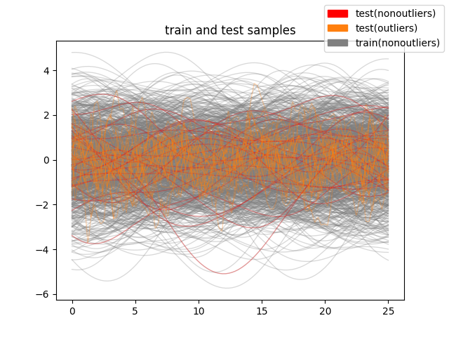
We plot the whole dataset.

whole_data = train_set.concatenate(test_set)
whole_data_labels = np.concatenate((train_set_labels, test_set_labels))

fig = whole_data.plot(
    group=whole_data_labels,
    group_colors={
        'train(nonoutliers)': 'grey',
        'test(nonoutliers)': 'red',
        'test(outliers)': 'C1'},
    linewidth=0.95,
    alpha=0.3,
    legend=True
)
plt.title('train and test samples')
fig.show()

We fit an FPCA with an arbitrary low number of components compared to the input dimension (grid size). We compute the relative RE of both the training and test samples, and plot the pdf estimates. Errors are normalized w.r.t L2-norms of each sample to remove (explained) variance from the scale error.

q = 5
fpca_clean = FPCA(n_components=q)
fpca_clean.fit(train_set)
train_set_hat = fpca_clean.inverse_transform(
    fpca_clean.transform(train_set)
)

err_train = l2_distance(
    train_set,
    train_set_hat
) / l2_norm(train_set)

test_set_hat = fpca_clean.inverse_transform(
    fpca_clean.transform(test_set)
)
err_test = l2_distance(
    test_set,
    test_set_hat
) / l2_norm(test_set)

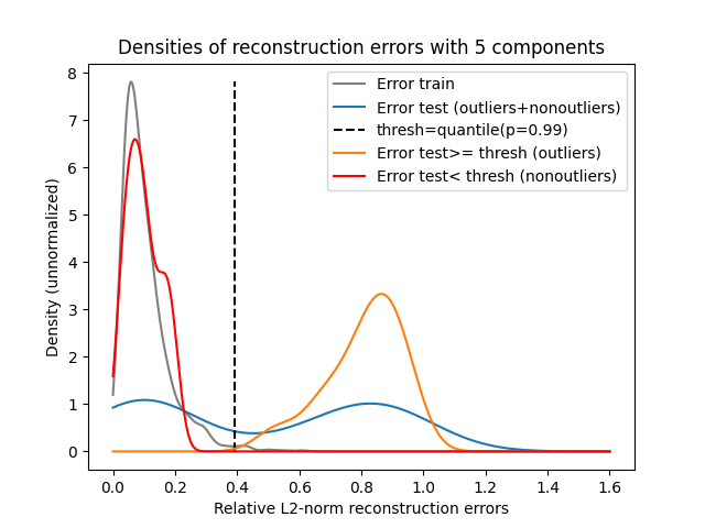
We plot the density of the REs, both unconditionaly (grey and blue) and conditionaly (orange and red), to the rule if error >= threshold then it is an outlier. The threshold is computed from RE of the training samples as the quantile of probability 0.99. In other words, a sample whose RE is higher than the threshold is unlikely approximated as a training sample, with probability 0.01.

x_density = np.linspace(0., 1.6, num=10**3)
density_train_err = gaussian_kde(err_train)
density_test_err = gaussian_kde(err_test)
err_thresh = np.quantile(err_train, 0.99)

density_test_err_outl = gaussian_kde(err_test[err_test >= err_thresh])
density_test_err_inli = gaussian_kde(err_test[err_test < err_thresh])

# density estimate of train errors
plt.plot(
    x_density,
    density_train_err(x_density),
    label='Error train',
    color='grey'
)

# density estimate of test errors
plt.plot(
    x_density,
    density_test_err(x_density),
    label='Error test (outliers+nonoutliers)',
    color='C0'
)

# outlyingness threshold
plt.vlines(
    err_thresh,
    ymax=max(density_train_err(x_density)),
    ymin=0.0,
    label='thresh=quantile(p=0.99)',
    linestyles='dashed',
    color='black'
)

# density estimate of the error of test samples flagged as outliers
plt.plot(
    x_density,
    density_test_err_outl(x_density),
    label='Error test>= thresh (outliers)',
    color='C1'
)

# density estimate of the error of test samples flagged as nonoutliers
plt.plot(
    x_density,
    density_test_err_inli(x_density),
    label='Error test< thresh (nonoutliers)',
    color='red'
)

plt.xlabel('Relative L2-norm reconstruction errors')
plt.ylabel('Density (unnormalized)')
plt.title(f'Densities of reconstruction errors with {q} components')
plt.legend()
plt.show()

We can check that the outliers are all detected with this method, with no false positive (wrongly) in the test set.

print('Flagged outliers: ')
print(test_set_labels[err_test >= err_thresh])
print('Flagged nonoutliers: ')
print(test_set_labels[err_test < err_thresh])

Flagged outliers:
['test(nonoutliers)' 'test(outliers)' 'test(outliers)' 'test(outliers)'
 'test(outliers)' 'test(outliers)' 'test(outliers)' 'test(outliers)'
 'test(outliers)' 'test(outliers)' 'test(outliers)' 'test(outliers)'
 'test(outliers)' 'test(outliers)' 'test(outliers)' 'test(outliers)'
 'test(outliers)' 'test(outliers)' 'test(outliers)' 'test(outliers)'
 'test(outliers)' 'test(outliers)' 'test(outliers)' 'test(outliers)'
 'test(outliers)' 'test(outliers)']
Flagged nonoutliers:
['test(nonoutliers)' 'test(nonoutliers)' 'test(nonoutliers)'
 'test(nonoutliers)' 'test(nonoutliers)' 'test(nonoutliers)'
 'test(nonoutliers)' 'test(nonoutliers)' 'test(nonoutliers)'
 'test(nonoutliers)' 'test(nonoutliers)' 'test(nonoutliers)'
 'test(nonoutliers)' 'test(nonoutliers)' 'test(nonoutliers)'
 'test(nonoutliers)' 'test(nonoutliers)' 'test(nonoutliers)'
 'test(nonoutliers)' 'test(nonoutliers)' 'test(nonoutliers)'
 'test(nonoutliers)' 'test(nonoutliers)' 'test(nonoutliers)']

We observe that the distribution of the training samples (grey) REs is unimodal and quite skewed toward 0. This means that the training samples are well recovered with 5 FPCs if we allow an reconsutrction error rate around 0.4. On the contrary, the distribution of the test samples (blue) REs is bimodal, where the two modes seem to be similar, meaning that half of the test samples is consistently approximated w.r.t training samples and the other half is poorly approximated in the FPCs basis.

The distribution underlying the left blue mode (red) is the one of test samples REs flagged as nonoutliers, i.e. having a RE_i<threshold. This means that test samples whose RE is low are effectively nonoutliers. Conversely, the distribution of REs underlying the right blue mode (orange) is the one of the test samples REs that we flagged as outliers.

To conclude this empirical example, the inverse_transform of FPCA can be used to detect outliers based on the magnitude of the REs compared to the training samples. Note that, here, an outlier is implicitly discriminated according to its covariance function. If a sample has a similar covariance function, compared to those of the training samples, it is very unlikely an outlier.