K-nearest neighbors classification

Shows the usage of the k-nearest neighbors classifier.

# Author: Pablo Marcos Manchón
# License: MIT

import matplotlib.pyplot as plt
import numpy as np
from sklearn.model_selection import GridSearchCV, train_test_split

import skfda
from skfda.ml.classification import KNeighborsClassifier

In this example we are going to show the usage of the K-nearest neighbors classifier in their functional version, which is a extension of the multivariate one, but using functional metrics.

Firstly, we are going to fetch a functional dataset, such as the Berkeley Growth Study. This dataset contains the height of several boys and girls measured until the 18 years of age. We will try to predict sex from their growth curves.

The following figure shows the growth curves grouped by sex.

X, y = skfda.datasets.fetch_growth(return_X_y=True, as_frame=True)
X = X.iloc[:, 0].values
y = y.values

# Plot samples grouped by sex
X.plot(group=y.codes, group_names=y.categories)

y = y.codes

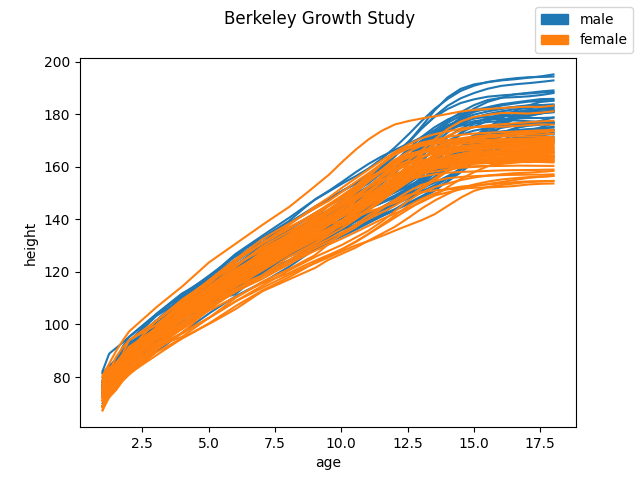
The class labels are stored in an array. Zeros represent male samples while ones represent female samples.

print(y)

[0 0 0 0 0 0 0 0 0 0 0 0 0 0 0 0 0 0 0 0 0 0 0 0 0 0 0 0 0 0 0 0 0 0 0 0 0
 0 0 1 1 1 1 1 1 1 1 1 1 1 1 1 1 1 1 1 1 1 1 1 1 1 1 1 1 1 1 1 1 1 1 1 1 1
 1 1 1 1 1 1 1 1 1 1 1 1 1 1 1 1 1 1 1]

We can split the dataset using the sklearn function train_test_split().

The function will return two FDataGrid’s, X_train and X_test with the corresponding partitions, and arrays with their class labels.

X_train, X_test, y_train, y_test = train_test_split(
    X,
    y,
    test_size=0.25,
    stratify=y,
    random_state=0,
)

We will fit the classifier KNeighborsClassifier with the training partition. This classifier works exactly like the sklearn multivariate classifier KNeighborsClassifier, but it’s input is a FDataGrid with functional observations instead of an array with multivariate data.

knn = KNeighborsClassifier(n_neighbors=5)
knn.fit(X_train, y_train)

KNeighborsClassifier()

In a Jupyter environment, please rerun this cell to show the HTML representation or trust the notebook.
On GitHub, the HTML representation is unable to render, please try loading this page with nbviewer.org.

Once it is fitted, we can predict labels for the test samples.

To predict the label of a test sample, the classifier will calculate the k-nearest neighbors and will assign the class shared by most of those k neighbors. In this case, we have set the number of neighbors to 5 (\(k=5\)). By default, it will use the \(\mathbb{L}^2\) distance between functions, to determine the neighborhood of a sample. However, it can be used with any of the functional metrics described in Metrics.

pred = knn.predict(X_test)
print(pred)

[0 0 1 0 1 1 1 0 0 0 0 1 1 0 0 0 0 1 1 1 1 1 1 1]

The score() method allows us to calculate the mean accuracy for the test data. In this case we obtained around 96% of accuracy.

score = knn.score(X_test, y_test)
print(score)

0.9583333333333334

We can also estimate the probability of membership to the predicted class using predict_proba(), which will return an array with the probabilities of the classes, in lexicographic order, for each test sample.

probs = knn.predict_proba(X_test[:5])  # Predict first 5 samples
print(probs)

[[1.  0. ]
 [0.6 0.4]
 [0.  1. ]
 [1.  0. ]
 [0.  1. ]]

We can use the sklearn GridSearchCV to perform a grid search to select the best hyperparams, using cross-validation.

In this case, we will vary the number of neighbors between 1 and 17.

# Only odd numbers, to prevent ties
param_grid = {"n_neighbors": range(1, 18, 2)}


knn = KNeighborsClassifier()

# Perform grid search with cross-validation
gscv = GridSearchCV(knn, param_grid, cv=5)
gscv.fit(X_train, y_train)


print("Best params:", gscv.best_params_)
print("Best cross-validation score:", gscv.best_score_)

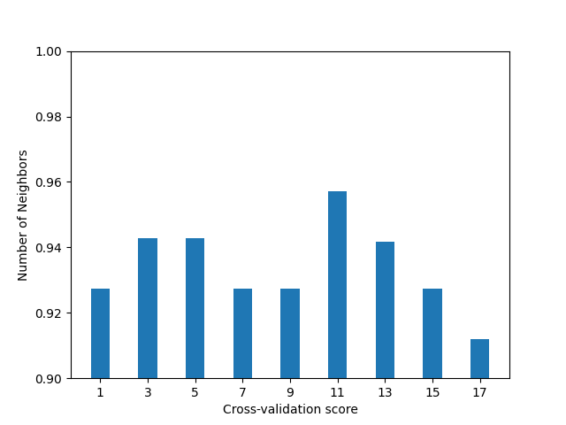
Best params: {'n_neighbors': 11}
Best cross-validation score: 0.9571428571428573

We have obtained the greatest mean accuracy using 11 neighbors. The following figure shows the score depending on the number of neighbors.

fig = plt.figure()
ax = fig.add_subplot(1, 1, 1)
ax.bar(param_grid["n_neighbors"], gscv.cv_results_["mean_test_score"])
ax.set_xticks(param_grid["n_neighbors"])
ax.set_ylabel("Number of Neighbors")
ax.set_xlabel("Cross-validation score")
ax.set_ylim((0.9, 1))

(0.9, 1.0)

By default, after performing the cross validation, the classifier will be fitted to the whole training data provided in the call to fit(). Therefore, to check the accuracy of the classifier for the number of neighbors selected (11), we can simply call the score() method.

score = gscv.score(X_test, y_test)
print(score)

1.0

This classifier can be used with multivariate functional data, as surfaces or curves in \(\mathbb{R}^N\), if the metric supports it too.