One-way functional ANOVA with real data

This example shows how to perform a functional one-way ANOVA test using a real dataset.

# Author: David García Fernández
# License: MIT

# sphinx_gallery_thumbnail_number = 4

import skfda
from skfda.inference.anova import oneway_anova
from skfda.representation.basis import FourierBasis

One-way ANOVA (analysis of variance) is a test that can be used to compare the means of different samples of data. Let \(X_{ij}(t), j=1, \dots, n_i\) be trajectories corresponding to \(k\) independent samples \((i=1,\dots,k)\) and let \(E(X_i(t)) = m_i(t)\). Thus, the null hypothesis in the statistical test is:

\[H_0: m_1(t) = \dots = m_k(t)\]

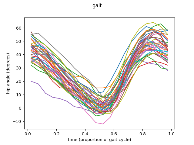
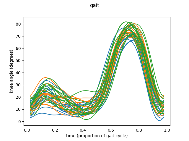
To illustrate this functionality we are going to explore the data available in GAIT dataset from fda R library. This dataset compiles a set of angles of hips and knees from 39 different boys in a 20 point movement cycle.

dataset = skfda.datasets.fetch_gait()
fd_hip = dataset['data'].coordinates[0]
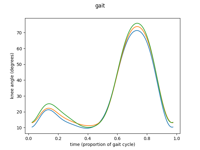
fd_knee = dataset['data'].coordinates[1].to_basis(FourierBasis(n_basis=10))

Let’s start with the first feature, the angle of the hip. The sample consists in 39 different trajectories, each representing the movement of the hip of each of the boys studied.

fig = fd_hip.plot()

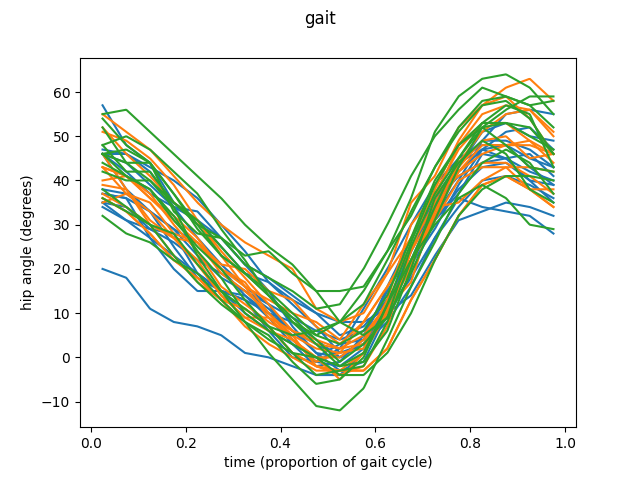
The example is going to be divided in three different groups. Then we are going to apply the ANOVA procedure to this groups to test if the means of this three groups are equal or not.

fd_hip1 = fd_hip[0:13]
fd_hip2 = fd_hip[13:26]
fd_hip3 = fd_hip[26:39]
fd_hip.plot(group=[0 if i < 13 else 1 if i < 26 else 39 for i in range(39)])

means = [fd_hip1.mean(), fd_hip2.mean(), fd_hip3.mean()]
fd_means = skfda.concatenate(means)
fig = fd_means.plot()

• 
• 

At this point is time to perform the ANOVA test. This functionality is implemented in the function oneway_anova(). As it consists in an asymptotic method it is possible to set the number of simulations necessary to approximate the result of the statistic. It is possible to set the \(p\) of the \(L_p\) norm used in the calculations (defaults 2).

v_n, p_val = oneway_anova(fd_hip1, fd_hip2, fd_hip3)

The function returns first the statistic v_sample_stat() used to measure the variability between groups, second the p-value of the test . For further information visit oneway_anova() and Cuevas et al.[1].

print('Statistic: ', v_n)
print('p-value: ', p_val)

Statistic:  368.0564102564103
p-value:  0.197

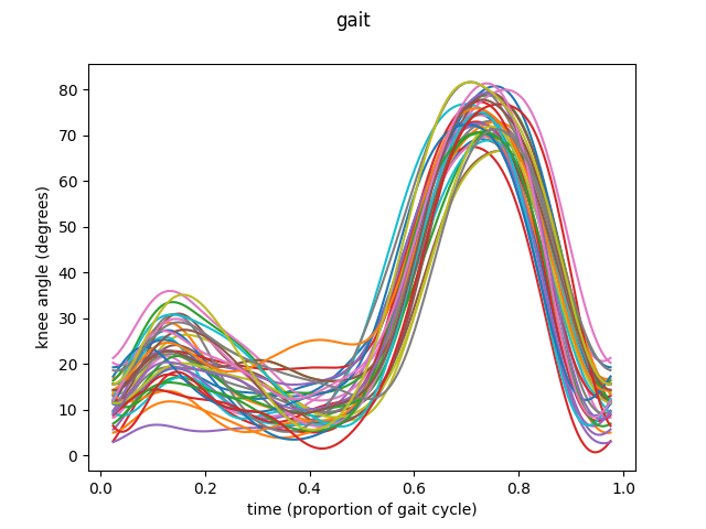
This was the simplest way to call this function. Let’s see another example, this time using knee angles, this time with data in basis representation.

fig = fd_knee.plot()

The same procedure as before is followed to prepare the data.

fd_knee1 = fd_knee[0:13]
fd_knee2 = fd_knee[13:26]
fd_knee3 = fd_knee[26:39]
fd_knee.plot(group=[0 if i < 13 else 1 if i < 26 else 39 for i in range(39)])

means = [fd_knee1.mean(), fd_knee2.mean(), fd_knee3.mean()]
fd_means = skfda.concatenate(means)
fig = fd_means.plot()

• 
• 

In this case the optional arguments of the function are going to be set. First, there is a n_reps parameter, which allows the user to select the number of simulations to perform in the asymptotic procedure of the test ( see oneway_anova()), defaults to 2000.

Also there is a p parameter to choose the \(p\) of the \(L_p\) norm used in the calculations (defaults 2).

Finally we can set to True the flag dist which allows the function to return a third value. This third return value corresponds to the sampling distribution of the statistic which is compared with the first return to get the p-value.

v_n, p_val, dist = oneway_anova(fd_knee1, fd_knee2, fd_knee3, n_reps=1500,
                                return_dist=True)

print('Statistic: ', v_n)
print('p-value: ', p_val)
print('Distribution: ', dist)

Statistic:  178.58753775850403
p-value:  0.528
Distribution:  [ 89.14740932 170.21382793 353.58745149 ...  64.09252303 100.97936004
  81.35847868]

References:

[1]

Antonio Cuevas, Manuel Febrero, and Ricardo Fraiman. An ANOVA test for functional data. Computational Statistics & Data Analysis, 47(1):111–122, August 2004. URL: http://www.sciencedirect.com/science/article/pii/S016794730300269X (visited on 2018-12-10), doi:10.1016/j.csda.2003.10.021.