Note

Go to the end to download the full example code or to run this example in your browser via Binder

Pairwise alignment#

Shows the usage of the elastic registration to perform a pairwise alignment.

# Author: Pablo Marcos Manchón
# License: MIT

# sphinx_gallery_thumbnail_number = 5


import matplotlib.colors as clr
import matplotlib.pyplot as plt
import numpy as np

import skfda
from skfda.datasets import make_multimodal_samples
from skfda.preprocessing.registration import (
    FisherRaoElasticRegistration,
    invert_warping,
)

Given any two functions \(f\) and \(g\), we define their pairwise alignment or registration to be the problem of finding a warping function \(\gamma^*\) such that a certain energy term \(E[f, g \circ \gamma]\) is minimized [1].

\[\gamma^*= \arg \min_{\gamma \in \Gamma} E[f \circ \gamma, g]\]

In the case of elastic registration it is taken as energy function the Fisher-Rao distance with a penalisation term, due to the property of invariance to reparameterizations of warpings functions [2].

\[E[f \circ \gamma, g] = d_{FR} (f \circ \gamma, g)\]

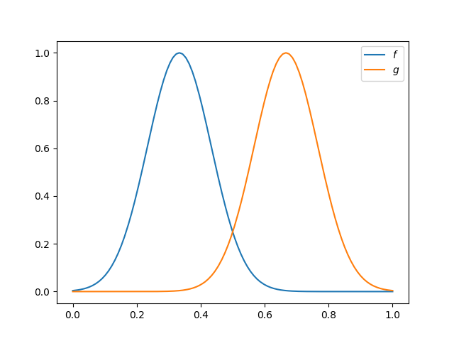
Firstly, we will create two unimodal samples, \(f\) and \(g\), defined in [0, 1] wich will be used to show the elastic registration. Due to the similarity of these curves can be aligned almost perfectly between them.

# Samples with modes in 1/3 and 2/3
fd = make_multimodal_samples(
    n_samples=2,
    modes_location=[1 / 3, 2 / 3],
    random_state=1,
    start=0,
    mode_std=0.01,
)

fig = fd.plot()
fig.axes[0].legend(['$f$', '$g$'])
plt.show()

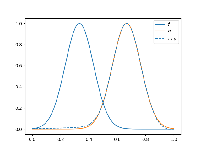
In this example \(g\) will be used as template and \(f\) will be aligned to it. In the following figure it is shown the result of the registration process, wich can be computed using FisherRaoElasticRegistration.

f, g = fd[0], fd[1]

elastic_registration = FisherRaoElasticRegistration(template=g)


# Aligns f to g
f_align = elastic_registration.fit_transform(f)

fig = fd.plot()
f_align.plot(fig=fig, color='C0', linestyle='--')


# Legend
fig.axes[0].legend(['$f$', '$g$', r'$f \circ \gamma $'])
plt.show()

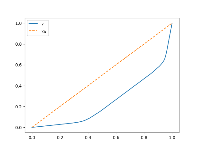
The non-linear transformation \(\gamma\) applied to \(f\) in the alignment is stored in the attribute warping_.

# Warping used in the last transformation
warping = elastic_registration.warping_
fig = warping.plot()

# Plot identity
t = np.linspace(0, 1)
fig.axes[0].plot(t, t, linestyle='--')

# Legend
fig.axes[0].legend([r'$\gamma$', r'$\gamma_{id}$'])
plt.show()

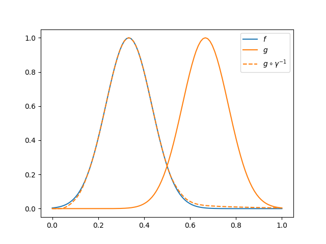
The transformation necessary to align \(g\) to \(f\) will be the inverse of the original warping function, \(\gamma^{-1}\). This fact is a consequence of the use of the Fisher-Rao metric as energy function.

warping_inverse = invert_warping(warping)

fig = fd.plot(label='$f$')
g.compose(warping_inverse).plot(fig=fig, color='C1', linestyle='--')


# Legend
fig.axes[0].legend(['$f$', '$g$', r'$g \circ \gamma^{-1} $'])
plt.show()

The amount of deformation used in the registration can be controlled by using a variation of the metric with a penalty term \(\lambda \mathcal{R}(\gamma)\) wich will reduce the elasticity of the metric.

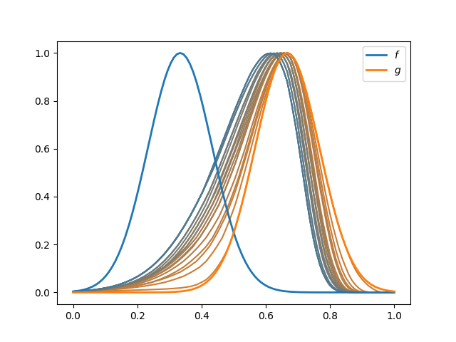
The following figure shows the original curves and the result to the alignment varying \(\lambda\) from 0 to 0.2.

# Values of lambda
penalties = np.linspace(0, 0.2, 20)

# Creation of a color gradient
cmap = clr.LinearSegmentedColormap.from_list('custom cmap', ['C1', 'C0'])
color = cmap(0.2 + 3 * penalties)

fig = plt.figure()
ax = fig.add_subplot(1, 1, 1)


for penalty, c in zip(penalties, color):

    elastic_registration.set_params(penalty=penalty)
    elastic_registration.transform(f).plot(fig, color=c)


f.plot(fig=fig, color='C0', linewidth=2, label='$f$')
g.plot(fig=fig, color='C1', linewidth=2, label='$g$')

# Legend
fig.axes[0].legend()
plt.show()

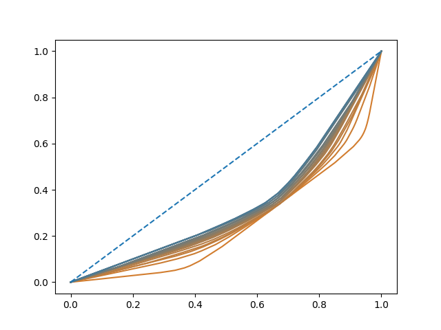
This phenomenon of loss of elasticity is clearly observed in the warpings used, since as the term of penalty increases, the functions are closer to \(\gamma_{id}\).

fig = plt.figure()
ax = fig.add_subplot(1, 1, 1)

for penalty, c in zip(penalties, color):
    elastic_registration.set_params(penalty=penalty)
    elastic_registration.transform(f)
    elastic_registration.warping_.plot(fig, color=c)

# Plots identity
fig.axes[0].plot(t, t, color='C0', linestyle="--")
plt.show()

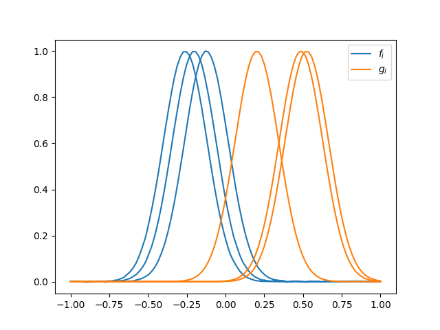
We can perform the pairwise of multiple curves at once. We can use a single curve as template to align a set of samples to it or a set of templates to make the alignemnt the two sets.

In the elastic registration example it is shown the alignment of multiple curves to the same template.

We will build two sets with 3 curves each, \(\{f_i\}\) and \(\{g_i\}\).

# Creation of the 2 sets of functions
state = np.random.RandomState(0)

location1 = state.normal(loc=-0.3, scale=0.1, size=3)
fd = skfda.datasets.make_multimodal_samples(
    n_samples=3,
    modes_location=location1,
    noise=0.001,
    random_state=1,
)

location2 = state.normal(
    loc=0.3,
    scale=0.1,
    size=3,
)
g = skfda.datasets.make_multimodal_samples(
    n_samples=3,
    modes_location=location2,
    random_state=2,
)

# Plot of the sets
fig = fd.plot(color="C0", label="$f_i$")
g.plot(fig=fig, color="C1", label="$g_i$")

labels = fig.axes[0].get_lines()
fig.axes[0].legend(handles=[labels[0], labels[-1]])
plt.show()

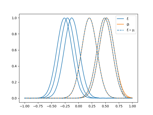
The following figure shows the result of the pairwise alignment of \(\{f_i\}\) to \(\{g_i\}\).

# Registration of the sets
elastic_registration = FisherRaoElasticRegistration(template=g)

fd_registered = elastic_registration.fit_transform(fd)

# Plot of the curves
fig = fd.plot(color="C0", label="$f_i$")
l1 = fig.axes[0].get_lines()[-1]
g.plot(fig=fig, color="C1", label="$g_i$")
l2 = fig.axes[0].get_lines()[-1]
fd_registered.plot(
    fig=fig,
    color="C0",
    linestyle="--",
    label=r"$f_i \circ \gamma_i$",
)
l3 = fig.axes[0].get_lines()[-1]

fig.axes[0].legend(handles=[l1, l2, l3])
plt.show()

Total running time of the script: (0 minutes 2.244 seconds)

Gallery generated by Sphinx-Gallery