Getting the data

In this section, we will dicuss how to get functional data to use in scikit-fda. We will briefly describe the FDataGrid class, which is the type that scikit-fda uses for storing and working with functional data in discretized form. We will discuss also how to import functional data from several sources and show how to fetch and load existing datasets popular in the FDA literature.

# Author: Carlos Ramos Carreño
# License: MIT
#
# sphinx_gallery_thumbnail_number = 6

The FDataGrid class

In order to use scikit-fda, first we need functional data to analyze. A common case is to have each functional observation measured at the same points. This kind of functional data is easily representable in scikit-fda using the FDataGrid class. The FDataGrid has two important attributes: data_matrix and grid_points.

The attribute grid_points is a tuple with the same length as the number of domain dimensions (that is, one for curves, two for surfaces…). Each of its elements is a 1D numpy ndarray containing the grid points for that particular dimension,

\[((t_{i 1}, \ldots, t_{i M_i}))_{i=1}^p,\]

where \(M_i\) is the number of measurement points for each “argument” or domain coordinate of the function \(i\) and \(p\) is the domain dimension.

The attribute data_matrix is a numpy ndarray containing the measured values of the functions in the grid spanned by the grid points. For functions \(\{x_n: \mathbb{R}^p \to \mathbb{R}^q\}_{n=1}^N\) this is a tensor with dimensions \(N \times M_1 \times \ldots \times M_p \times q\).

In order to create a FDataGrid, these attributes may be provided. The attributes are converted to ndarray when necessary.

Note

The grid points can be omitted, and in that case their number is inferred from the dimensions of data_matrix and they are automatically assigned as equispaced points in the unitary cube in the domain set.

In the common case of functions with domain dimension of 1, the list of grid points can be passed directly as grid_points.

If the codomain dimension is 1, the last dimension of data_matrix can be dropped.

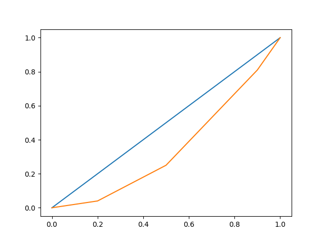
The following example shows the creation of a FDataGrid with two functions (curves) \(\{x_i: \mathbb{R} \to \mathbb{R}\}, i=1,2\) measured at the same (non-equispaced) points.

import skfda
import matplotlib.pyplot as plt

grid_points = [0, 0.2, 0.5, 0.9, 1]  # Grid points of the curves
data_matrix = [
    [0, 0.2, 0.5, 0.9, 1],     # First observation
    [0, 0.04, 0.25, 0.81, 1],  # Second observation
]

fd = skfda.FDataGrid(
    data_matrix=data_matrix,
    grid_points=grid_points,
)

fd.plot()
plt.show()

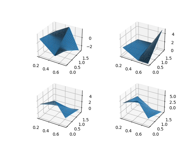
Advanced example

In order to better understand the FDataGrid structure, you can consider the following example, in which a FDataGrid object is created, containing just one function (vector-valued surface) \(x: \mathbb{R}^2 \to \mathbb{R}^4\).

grid_points_surface = [
    [0.2, 0.5, 0.7],      # Measurement points in first domain dimension
    [0, 1.5],             # Measurement points in second domain dimension
]

data_matrix_surface = [
    # First observation
    [
        # 0.2
        [
            # Value at (0.2, 0)
            [1, 2, 3, 4.1],
            # Value at (0.2, 1.5)
            [0, 1, -1.3, 2],
        ],
        # 0.5
        [
            # Value at (0.5, 0)
            [-2, 0, 5.5, 7],
            # Value at (0.5, 1.5)
            [2, 1.1, -1, -2],
        ],
        # 0.7
        [
            # Value at (0.7, 0)
            [0, 0, 1.1, 1],
            # Value at (0.7, 1.5)
            [-3, 5, -0.5, -2],
        ],
    ],
    # This example has only one observation. Next observations would be
    # added here.
]

fd = skfda.FDataGrid(
    data_matrix=data_matrix_surface,
    grid_points=grid_points_surface,
)

fd.plot()
plt.show()

Importing data

Usually the data used in the analysis comes from previous measurements of an experiment, that have been stored in some file format, such as comma-separated values (CSV), attribute-relation file format (ARFF) or Matlab and R formats. Users should know the particular layout used for representing functional data on their files, as there is currently no standard format for storing this kind of data.

Note

scikit-fda does not offer input/output functions right now. You can parse the grid points and values of the functions using the available tools in the Scientific Python ecosystem:

• Numpy: for simple text-based or binary formats, such as CSV.

• Scipy: for Matlab, Fortran or ARFF files.

• RData: for loading data in the R file formats.

• Pandas: includes tools for reading a variety of file formats, such as CSV, JSON, HTML, LaTeX, XML, Excel, HDF5, Parquet, SPSS or SQL.

Once the data is loaded as NumPy arrays, you can construct the FDataGrid as explained above.

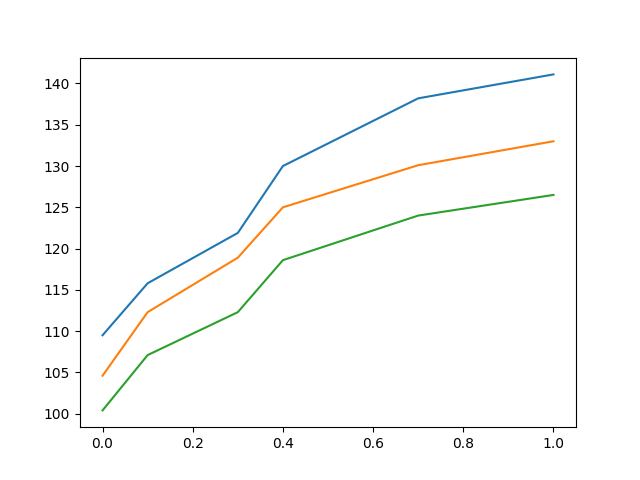
For example, consider the following file, containing unidimensional functional data in CSV form. The first row (the header) contains the grid points, common for all observations. Each of the following rows is a functional observation.

import pathlib
import textwrap

file_content = textwrap.dedent(
    """\
    0.0, 0.1, 0.3, 0.4, 0.7, 1.0
    109.5, 115.8, 121.9, 130.0, 138.2, 141.1
    104.6, 112.3, 118.9, 125.0, 130.1, 133.0
    100.4, 107.1, 112.3, 118.6, 124.0, 126.5
    """,
)

test_file = pathlib.Path("data.csv")
test_file.write_text(file_content)
text = test_file.read_text()
print(text)

0.0, 0.1, 0.3, 0.4, 0.7, 1.0
109.5, 115.8, 121.9, 130.0, 138.2, 141.1
104.6, 112.3, 118.9, 125.0, 130.1, 133.0
100.4, 107.1, 112.3, 118.6, 124.0, 126.5

We can now load the CSV using the functions in Pandas. Note that by default, Pandas reads the header as text and uses it to name the columns. Thus, we need to convert it to float before we can pass it to the FDataGrid constructor.

import pandas

data = pandas.read_csv("data.csv")

grid_points = data.columns.astype(float)
data_matrix = data

We can now construct the FDataGrid as before and plot it:

fd = skfda.FDataGrid(
    data_matrix=data_matrix,
    grid_points=grid_points,
)

fd.plot()
plt.show()

If you have data that is already a NumPy array, you can use it directly. For example, we will load the digits dataset of scikit-learn, which is a preprocessed subset of the MNIST dataset, containing digit images. The data is already a NumPy array. As the data has been flattened into a 1D vector of pixels, we need to reshape the arrays to their original 8x8 shape. Then this array can be used to construct the digits as surfaces.

from sklearn.datasets import load_digits

X, y = load_digits(return_X_y=True)
X = X.reshape(-1, 8, 8)

fd = skfda.FDataGrid(X)

# Plot the first 2 observations
fd[0].plot()
fd[1].plot()
plt.show()

• 
• 

Common datasets

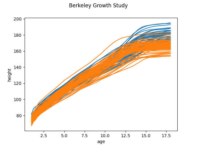
scikit-fda can download and import for you several of the most popular datasets in the FDA literature, such as the Berkeley Growth dataset (function fetch_growth()) or the Canadian Weather dataset (function fetch_weather()). These datasets are often useful as benchmarks, in order to compare results between different algorithms, or simply as examples to use in teaching or research.

X, y = skfda.datasets.fetch_growth(return_X_y=True)

X.plot(group=y)
plt.show()

Datasets from CRAN

If you want to work with a dataset for which no fetching function exist, and you know that is available inside a R package in the CRAN repository, you can try using the function fetch_cran(). This function will load the package, fetch the dataset and convert it to Python objects using the packages scikit-datasets and RData. As datasets in CRAN follow no particular structure, you will need to know how it is structured internally in order to use it properly.

Note

Functional data objects from some packages, such as fda.usc are automatically recognized as such and converted to FDataGrid instances. This behaviour can be disabled or customized to work with more packages.

data = skfda.datasets.fetch_cran("MCO", "fda.usc")

data["MCO"]["intact"].plot()
plt.show()

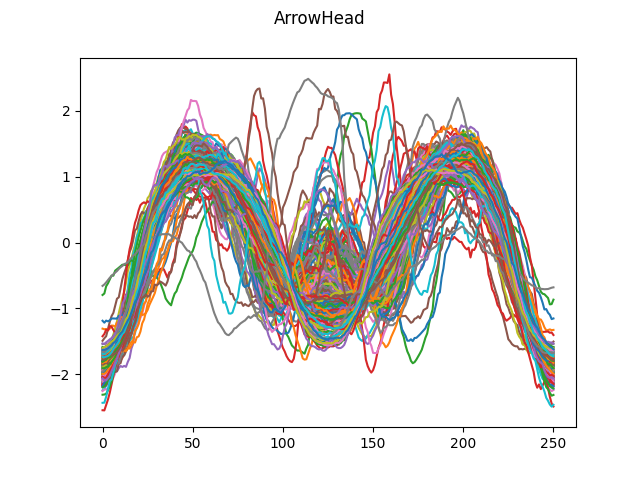
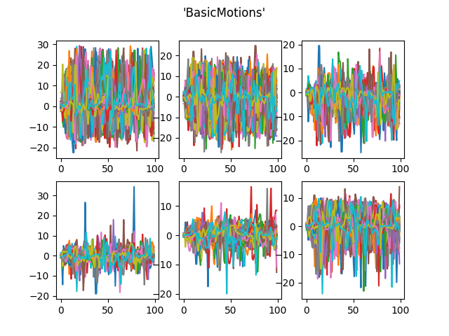
Datasets from the UEA & UCR Time Series Classification Repository

The UEA & UCR Time Series Classification Repository is a popular repository for classification problems involving time series data. The datasets used can be considered also as functional observations, where the functions involved have domain dimension of 1, and the grid points are equispaced. Thus, they have also been used in the FDA literature. The original UCR datasets are univariate time series, while the new UEA datasets incorporate also vector-valued data. In scikit-fda, the function fetch_ucr() can be used to obtain both kinds of datasets as FDataGrid instances.

# Load ArrowHead dataset from UCR
dataset = skfda.datasets.fetch_ucr("ArrowHead")
dataset["data"].plot()
plt.show()

# Load BasicMotions dataset from UEA
dataset = skfda.datasets.fetch_ucr("BasicMotions")
dataset["data"].plot()
plt.show()

Synthetic data

Sometimes it is not enough to have real-world data at your disposal. Perhaps the messy nature of real-world data makes difficult to detect when a particular algorithm has a strange behaviour. Perhaps you want to see how it performs under a simplified model. Maybe you want to see what happens when your data has particular characteristics, for which no dataset is available. Or maybe you only want to illustrate a concept without having to introduce a particular set of data.

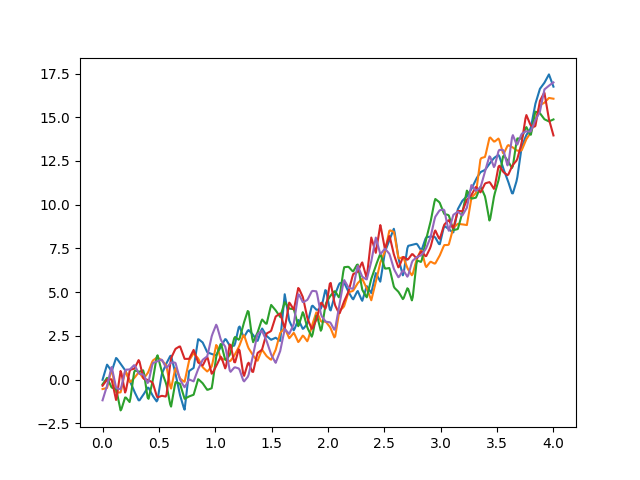
In those cases, the ability to use generated data is desirable. To aid this use case, scikit-learn provides several functions that generate data according to some model. These functions are in the datasets module and have the prefix make_. Maybe the most useful of those are the functions skfda.datasets.make_gaussian_process() and skfda.datasets.make_gaussian() which can be used to generate Gaussian processes and Gaussian fields with different covariance functions.

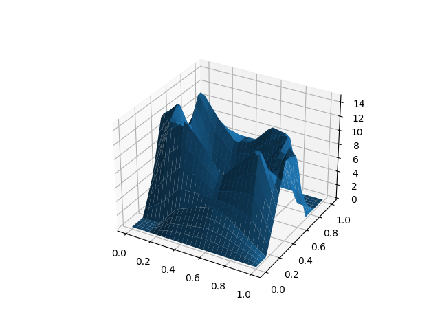
cov = skfda.misc.covariances.Exponential(length_scale=0.1)

fd = skfda.datasets.make_gaussian_process(
    start=0,
    stop=4,
    n_samples=5,
    n_features=100,
    mean=lambda t: t**2,
    cov=cov,
)

fd.plot()
plt.show()

In order to know all the available functionalities to load existing and synthetic datasets it is recommended to look at the documentation of the datasets module.