LinearRegression#
- class skfda.ml.regression.LinearRegression(*, coef_basis=None, fit_intercept=True, regularization=None)[source]#
Linear regression with multivariate and functional response.
This is a regression algorithm equivalent to multivariate linear regression, but accepting also functional data expressed in a basis expansion.
Functional linear regression model is subdivided into three broad categories, depending on whether the responses or the covariates, or both, are curves.
Particulary, when the response is scalar, the model assumed is:
\[y = w_0 + w_1 x_1 + \ldots + w_p x_p + \int w_{p+1}(t) x_{p+1}(t) dt \ + \ldots + \int w_r(t) x_r(t) dt\]where the covariates can be either multivariate or functional and the response is multivariate.
When the response is functional, the model assumed is:
\[y(t) = \boldsymbol{X} \boldsymbol{\beta}(t)\]where the covariates are multivariate and the response is functional; or:
\[y(t) = \boldsymbol{X}(t) \boldsymbol{\beta}(t)\]if the model covariates are also functional (concurrent).
Deprecated since version 0.8.: Usage of arguments of type sequence of FData, ndarray is deprecated in methods fit, predict. Use covariate parameters of type pandas.DataFrame instead.
Warning
For now, only multivariate and concurrent convariates are supported when the response is functional.
Warning
This functionality is still experimental. Users should be aware that the API will suffer heavy changes in the future.
- Parameters:
coef_basis (iterable) – Basis of the coefficient functions of the functional covariates. When the response is scalar, if multivariate data is supplied, their corresponding entries should be
None. IfNoneis provided for a functional covariate, the same basis is assumed. If this parameter isNone(the default), it is assumed thatNoneis provided for all covariates. When the response is functional, ifNoneis provided, the response basis is used for all covariates.fit_intercept (bool) – Whether to calculate the intercept for this model. If set to False, no intercept will be used in calculations (i.e. data is expected to be centered). When the response is functional, a coef_basis for intercept must be supplied.
regularization (int, iterable or
Regularization) – If it is not aRegularizationobject, linear differential operator regularization is assumed. If it is an integer, it indicates the order of the derivative used in the computing of the penalty matrix. For instance 2 means that the differential operator is \(f''(x)\). If it is an iterable, it consists on coefficients representing the differential operator used in the computing of the penalty matrix. For instance the tuple (1, 0, numpy.sin) means \(1 + sin(x)D^{2}\). If not supplied this defaults to 2. Only used if penalty_matrix isNone.
- Attributes:
coef_ – A list containing the weight coefficient for each covariate.
intercept_ – Independent term in the linear model. Set to 0.0 if fit_intercept = False.
Examples
Functional linear regression can be used with functions expressed in a basis. Also, a functional basis for the weights can be specified:
>>> from skfda.ml.regression import LinearRegression
>>> from skfda.representation.basis import (
...     FDataBasis,
...     MonomialBasis,
...     ConstantBasis,
... )
>>> x_basis = MonomialBasis(n_basis=3)
>>> X_train = FDataBasis(
...     basis=x_basis,
...     coefficients=[
...         [0, 0, 1],
...         [0, 1, 0],
...         [0, 1, 1],
...         [1, 0, 1],
...     ],
... )
>>> y_train = [2, 3, 4, 5]
>>> X_test = X_train  # Just for illustration purposes
>>> linear_reg = LinearRegression()
>>> _ = linear_reg.fit(X_train, y_train)
>>> linear_reg.coef_[0]
FDataBasis(
    basis=MonomialBasis(domain_range=((0.0, 1.0),), n_basis=3),
    coefficients=[[-15.  96. -90.]],
    ...)
>>> linear_reg.intercept_
array([ 1.])
>>> linear_reg.predict(X_test)
array([ 2.,  3.,  4.,  5.])
Covariates can include also multivariate data. In order to mix functional and multivariate data a dataframe can be used:
>>> import pandas as pd
>>> x_basis = MonomialBasis(n_basis=2)
>>> X_train = pd.DataFrame({
...     "functional_covariate": FDataBasis(
...         basis=x_basis,
...         coefficients=[
...             [0, 2],
...             [0, 4],
...             [1, 0],
...             [2, 0],
...             [1, 2],
...             [2, 2],
...         ]
...     ),
...     "multivariate_covariate_1": [1, 2, 4, 1, 3, 2],
...     "multivariate_covariate_2": [7, 3, 2, 1, 1, 5],
... })
>>> y_train = [11, 10, 12, 6, 10, 13]
>>> X_test = X_train  # Just for illustration purposes
>>> linear_reg = LinearRegression(
...     coef_basis=[ConstantBasis(), None, None],
... )
>>> _ = linear_reg.fit(X_train, y_train)
>>> linear_reg.coef_[0]
FDataBasis(
    basis=ConstantBasis(domain_range=((0.0, 1.0),), n_basis=1),
    coefficients=[[ 1.]],
    ...)
>>> linear_reg.coef_[1]
array([ 2.])
>>> linear_reg.coef_[2]
array([ 1.])
>>> linear_reg.intercept_
array([ 1.])
>>> linear_reg.predict(X_test)
array([ 11.,  10.,  12.,   6.,  10.,  13.])
Response can be functional when covariates are multivariate:
>>> y_basis = MonomialBasis(n_basis=3)
>>> X_train = pd.DataFrame({
...     "covariate_1": [3, 5, 3],
...     "covariate_2": [4, 1, 2],
...     "covariate_3": [1, 6, 8],
... })
>>> y_train = FDataBasis(
...     basis=y_basis,
...     coefficients=[
...         [47, 22, 24],
...         [43, 47, 39],
...         [40, 53, 51],
...     ],
... )
>>> X_test = X_train  # Just for illustration purposes
>>> linear_reg = LinearRegression(
...     regularization=None,
...     fit_intercept=False,
... )
>>> _ = linear_reg.fit(X_train, y_train)
>>> linear_reg.coef_[0]
FDataBasis(
    basis=MonomialBasis(domain_range=((0.0, 1.0),), n_basis=3),
    coefficients=[[ 6.  3.  1.]],
    ...)
>>> linear_reg.predict(X_test)
FDataBasis(
    basis=MonomialBasis(domain_range=((0.0, 1.0),), n_basis=3),
    coefficients=[[ 47. 22. 24.]
        [ 43. 47. 39.]
        [ 40. 53. 51.]],
     ...)
Concurrent function-on-function regression is also supported:
>>> x_basis = MonomialBasis(n_basis=3)
>>> y_basis = MonomialBasis(n_basis=2)
>>> X_train = FDataBasis(
...     basis=x_basis,
...     coefficients=[
...         [0, 1, 0],
...         [2, 1, 0],
...         [5, 0, 1],
...     ],
... )
>>> y_train = FDataBasis(
...     basis=y_basis,
...     coefficients=[
...         [1, 1],
...         [2, 1],
...         [3, 1],
...     ],
... )
>>> X_test = X_train  # Just for illustration purposes
>>> linear_reg = LinearRegression(
...     coef_basis=[y_basis],
...     fit_intercept=False,
... )
>>> _ = linear_reg.fit(X_train, y_train)
>>> linear_reg.coef_[0]
FDataBasis(
    basis=MonomialBasis(domain_range=((0.0, 1.0),), n_basis=2),
    coefficients=[[ 0.68250377  0.09960705]],
    ...)
>>> linear_reg.predict(X_test)
FDataBasis(
    basis=MonomialBasis(domain_range=((0.0, 1.0),), n_basis=2),
    coefficients=[[-0.01660117  0.78211082]
        [ 1.34840637  0.98132492]
        [ 3.27884682  1.27018536]],
     ...)
Methods
fit(X, y[, sample_weight])Get metadata routing of this object.
get_params([deep])Get parameters for this estimator.
predict(X)score(X, y[, sample_weight])Return the coefficient of determination of the prediction.
set_fit_request(*[, sample_weight])Request metadata passed to the
fitmethod.set_params(**params)Set the parameters of this estimator.
set_score_request(*[, sample_weight])Request metadata passed to the
scoremethod.- get_metadata_routing()#
Get metadata routing of this object.
Please check User Guide on how the routing mechanism works.
- Returns:
routing – A
MetadataRequestencapsulating routing information.- Return type:
MetadataRequest
- get_params(deep=True)#
Get parameters for this estimator.
- score(X, y, sample_weight=None)[source]#
Return the coefficient of determination of the prediction.
The coefficient of determination \(R^2\) is defined as \((1 - \frac{u}{v})\), where \(u\) is the residual sum of squares
((y_true - y_pred)** 2).sum()and \(v\) is the total sum of squares((y_true - y_true.mean()) ** 2).sum(). The best possible score is 1.0 and it can be negative (because the model can be arbitrarily worse). A constant model that always predicts the expected value of y, disregarding the input features, would get a \(R^2\) score of 0.0.- Parameters:
X (array-like of shape (n_samples, n_features)) – Test samples. For some estimators this may be a precomputed kernel matrix or a list of generic objects instead with shape
(n_samples, n_samples_fitted), wheren_samples_fittedis the number of samples used in the fitting for the estimator.y (array-like of shape (n_samples,) or (n_samples, n_outputs)) – True values for X.
sample_weight (array-like of shape (n_samples,), default=None) – Sample weights.
- Returns:
score – \(R^2\) of
self.predict(X)w.r.t. y.- Return type:
Notes
The \(R^2\) score used when calling
scoreon a regressor usesmultioutput='uniform_average'from version 0.23 to keep consistent with default value ofr2_score(). This influences thescoremethod of all the multioutput regressors (except forMultiOutputRegressor).
- set_fit_request(*, sample_weight='$UNCHANGED$')#
Request metadata passed to the
fitmethod.Note that this method is only relevant if
enable_metadata_routing=True(seesklearn.set_config()). Please see User Guide on how the routing mechanism works.The options for each parameter are:
True: metadata is requested, and passed tofitif provided. The request is ignored if metadata is not provided.False: metadata is not requested and the meta-estimator will not pass it tofit.None: metadata is not requested, and the meta-estimator will raise an error if the user provides it.str: metadata should be passed to the meta-estimator with this given alias instead of the original name.
The default (
sklearn.utils.metadata_routing.UNCHANGED) retains the existing request. This allows you to change the request for some parameters and not others.Added in version 1.3.
Note
This method is only relevant if this estimator is used as a sub-estimator of a meta-estimator, e.g. used inside a
Pipeline. Otherwise it has no effect.- Parameters:
sample_weight (str, True, False, or None, default=sklearn.utils.metadata_routing.UNCHANGED) – Metadata routing for
sample_weightparameter infit.self (LinearRegression)
- Returns:
self – The updated object.
- Return type:
- set_params(**params)#
Set the parameters of this estimator.
The method works on simple estimators as well as on nested objects (such as
Pipeline). The latter have parameters of the form<component>__<parameter>so that it’s possible to update each component of a nested object.- Parameters:
**params (dict) – Estimator parameters.
- Returns:
self – Estimator instance.
- Return type:
estimator instance
- set_score_request(*, sample_weight='$UNCHANGED$')#
Request metadata passed to the
scoremethod.Note that this method is only relevant if
enable_metadata_routing=True(seesklearn.set_config()). Please see User Guide on how the routing mechanism works.The options for each parameter are:
True: metadata is requested, and passed toscoreif provided. The request is ignored if metadata is not provided.False: metadata is not requested and the meta-estimator will not pass it toscore.None: metadata is not requested, and the meta-estimator will raise an error if the user provides it.str: metadata should be passed to the meta-estimator with this given alias instead of the original name.
The default (
sklearn.utils.metadata_routing.UNCHANGED) retains the existing request. This allows you to change the request for some parameters and not others.Added in version 1.3.
Note
This method is only relevant if this estimator is used as a sub-estimator of a meta-estimator, e.g. used inside a
Pipeline. Otherwise it has no effect.- Parameters:
sample_weight (str, True, False, or None, default=sklearn.utils.metadata_routing.UNCHANGED) – Metadata routing for
sample_weightparameter inscore.self (LinearRegression)
- Returns:
self – The updated object.
- Return type:
Examples using skfda.ml.regression.LinearRegression#
Functional Linear Regression with multivariate covariates.
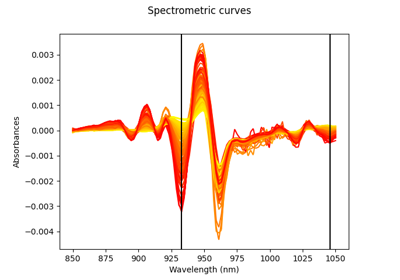
Spectrometric data: derivatives, regression, and variable selection