MagnitudeShapePlot#
- class skfda.exploratory.visualization.MagnitudeShapePlot(fdata, chart=None, *, fig=None, axes=None, ellipsoid=True, **kwargs)[source]#
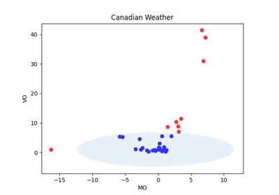
Implementation of the magnitude-shape plot.
This plot, which is based on the calculation of the
directional
outlyingness
of each of the samples, serves as a visualization tool for the centrality of curves. Furthermore, an outlier detection procedure is included.The norm of the mean of the directional outlyingness (\(\lVert \mathbf{MO}\rVert\)) is plotted in the x-axis, and the variation of the directional outlyingness (\(VO\)) in the y-axis.
The outliers are detected using an instance of
MSPlotOutlierDetector.For more information see Dai and Genton[1].
- Parameters:
fdata (FDataGrid) – Object containing the data.
multivariate_depth – Method used to order the data. Defaults to
projection depth.pointwise_weights – an array containing the weights of each points of discretisation where values have been recorded.
cutoff_factor – Factor that multiplies the cutoff value, in order to consider more or less curves as outliers.
assume_centered – If True, the support of the robust location and the covariance estimates is computed, and a covariance estimate is recomputed from it, without centering the data. Useful to work with data whose mean is significantly equal to zero but is not exactly zero. If False, default value, the robust location and covariance are directly computed with the FastMCD algorithm without additional treatment.
support_fraction – The proportion of points to be included in the support of the raw MCD estimate. Default is None, which implies that the minimum value of support_fraction will be used within the algorithm: [n_sample + n_features + 1] / 2
random_state – If int, random_state is the seed used by the random number generator; If RandomState instance, random_state is the random number generator; If None, the random number generator is the RandomState instance used by np.random. By default, it is 0.
ellipsoid (bool) – Whether to draw the non outlying ellipsoid.
chart (Figure | Axes | None)
fig (Figure | None)
axes (Sequence[Axes] | None)
kwargs (Any)
- Attributes:
points (numpy.ndarray) – 2-dimensional matrix where each row contains the points plotted in the graph.
outliers (1-D array, (fdata.n_samples,)) – Contains 1 or 0 to denote if a sample is an outlier or not, respecively.
colormap (matplotlib.pyplot.LinearSegmentedColormap, optional) – Colormap from which the colors of the plot are extracted. Defaults to ‘seismic’.
color (float, optional) – Tone of the colormap in which the nonoutlier points are plotted. Defaults to 0.2.
outliercol (float, optional) – Tone of the colormap in which the outliers are plotted. Defaults to 0.8.
xlabel (string, optional) – Label of the x-axis. Defaults to ‘MO’, mean of the directional outlyingness.
ylabel (string, optional) – Label of the y-axis. Defaults to ‘VO’, variation of the directional outlyingness.
title (string, optional) – Title of the plot. defaults to ‘MS-Plot’.
Representation in a Jupyter notebook:
from skfda.datasets import make_gaussian_process
from skfda.misc.covariances import Exponential
from skfda.exploratory.visualization import MagnitudeShapePlot

X = make_gaussian_process(
        n_samples=20, cov=Exponential(), random_state=1)

MagnitudeShapePlot(X)

Example
>>> import skfda
>>> data_matrix = [[1, 1, 2, 3, 2.5, 2],
...                [0.5, 0.5, 1, 2, 1.5, 1],
...                [-1, -1, -0.5, 1, 1, 0.5],
...                [-0.5, -0.5, -0.5, -1, -1, -1]]
>>> grid_points = [ 0., 2., 4., 6., 8., 10.]
>>> X = skfda.FDataGrid(data_matrix, grid_points)
>>> MagnitudeShapePlot(X)
MagnitudeShapePlot(...)
References
Methods
- hover(event)[source]#
Activate the annotation when hovering a point.
Callback method that activates the annotation when hovering a specific point in a graph. The annotation is a description of the point containing its coordinates.
- Parameters:
event (MouseEvent) – event object containing the artist of the point hovered.
- Return type:
None
Examples using skfda.exploratory.visualization.MagnitudeShapePlot#
Meteorological data: data visualization, clustering, and functional PCA