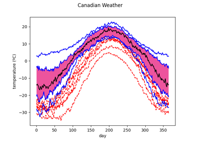
Boxplot#
- class skfda.exploratory.visualization.Boxplot(fdatagrid, chart=None, *, depth_method=None, prob=(0.5,), factor=1.5, fig=None, axes=None, n_rows=None, n_cols=None)[source]#
Representation of the functional boxplot.
Class implementing the functionl boxplot which is an informative exploratory tool for visualizing functional data, as well as its generalization, the enhanced functional boxplot. Only supports 1 dimensional domain functional data.
Based on the center outward ordering induced by a depth measure for functional data, the descriptive statistics of a functional boxplot are: the envelope of the 50% central region, the median curve,and the maximum non-outlying envelope. In addition, outliers can be detected in a functional boxplot by the 1.5 times the 50% central region empirical rule, analogous to the rule for classical boxplots.
For more information see Sun and Genton[1].
- Parameters:
fdatagrid (FData) – Object containing the data.
chart (Figure | Axes | None) – figure over with the graphs are plotted or axis over where the graphs are plotted. If None and ax is also None, the figure is initialized.
depth_method (Depth[FDataGrid] | None) – Method used to order the data. Defaults to
ModifiedBandDepth().prob (Sequence[float]) – List with float numbers (in the range from 1 to 0) that indicate which central regions to represent. Defaults to (0.5,) which represents the 50% central region.
factor (float) – Number used to calculate the outlying envelope.
fig (Figure | None) – Figure over with the graphs are plotted in case ax is not specified. If None and ax is also None, the figure is initialized.
axes (Axes | None) – Axis over where the graphs are plotted. If None, see param fig.
n_rows (int | None) – Designates the number of rows of the figure to plot the different dimensions of the image. Only specified if fig and ax are None.
n_cols (int | None) – Designates the number of columns of the figure to plot the different dimensions of the image. Only specified if fig and ax are None.
- Attributes:
fdatagrid – Object containing the data.
median – Contains the median/s.
central_envelope – Contains the central envelope/s.
non_outlying_envelope – Contains the non-outlying envelope/s.
colormap – Colormap from which the colors to represent the central regions are selected.
envelopes – Contains the region envelopes.
outliers – Contains the outliers.
barcol – Color of the envelopes and vertical lines.
outliercol – Color of the ouliers.
mediancol – Color of the median.
show_full_outliers – If False (the default) then only the part outside the box is plotted. If True, complete outling curves are plotted.
Representation in a Jupyter notebook:
from skfda.datasets import make_gaussian_process
from skfda.misc.covariances import Exponential
from skfda.exploratory.visualization import Boxplot

fd = make_gaussian_process(
        n_samples=20, cov=Exponential(), random_state=3)

Boxplot(fd)

Examples
Function \(f : \mathbb{R}\longmapsto\mathbb{R}\).
>>> from skfda import FDataGrid
>>> from skfda.exploratory.visualization import Boxplot
>>>
>>> data_matrix = [[1, 1, 2, 3, 2.5, 2],
...                [0.5, 0.5, 1, 2, 1.5, 1],
...                [-1, -1, -0.5, 1, 1, 0.5],
...                [-0.5, -0.5, -0.5, -1, -1, -1]]
>>> grid_points = [0, 2, 4, 6, 8, 10]
>>> fd = FDataGrid(data_matrix, grid_points, dataset_name="dataset",
...                argument_names=["x_label"],
...                coordinate_names=["y_label"])
>>> Boxplot(fd)
Boxplot(
    FDataGrid=FDataGrid(
        array([[[ 1. ],
                [ 1. ],
                [ 2. ],
                [ 3. ],
                [ 2.5],
                [ 2. ]],
               [[ 0.5],
                [ 0.5],
                [ 1. ],
                [ 2. ],
                [ 1.5],
                [ 1. ]],
               [[-1. ],
                [-1. ],
                [-0.5],
                [ 1. ],
                [ 1. ],
                [ 0.5]],
               [[-0.5],
                [-0.5],
                [-0.5],
                [-1. ],
                [-1. ],
                [-1. ]]]),
        grid_points=(array([ 0.,  2.,  4.,  6.,  8., 10.]),),
        domain_range=((0.0, 10.0),),
        dataset_name='dataset',
        argument_names=('x_label',),
        coordinate_names=('y_label',),
        ...),
    median=array([[ 0.5],
                  [ 0.5],
                  [ 1. ],
                  [ 2. ],
                  [ 1.5],
                  [ 1. ]]),
    central envelope=(array([[-1. ],
                             [-1. ],
                             [-0.5],
                             [ 1. ],
                             [ 1. ],
                             [ 0.5]]), array([[ 0.5],
                             [ 0.5],
                             [ 1. ],
                             [ 2. ],
                             [ 1.5],
                             [ 1. ]])),
    non-outlying envelope=(array([[-1. ],
                                  [-1. ],
                                  [-0.5],
                                  [ 1. ],
                                  [ 1. ],
                                  [ 0.5]]), array([[ 0.5],
                                  [ 0.5],
                                  [ 1. ],
                                  [ 2. ],
                                  [ 1.5],
                                  [ 1. ]])),
    envelopes=[(array([[-1. ],
                       [-1. ],
                       [-0.5],
                       [ 1. ],
                       [ 1. ],
                       [ 0.5]]), array([[ 0.5],
                       [ 0.5],
                       [ 1. ],
                       [ 2. ],
                       [ 1.5],
                       [ 1. ]]))],
    outliers=array([ True, False, False,  True]))
References
Methods
- hover(event)[source]#
Activate the annotation when hovering a point.
Callback method that activates the annotation when hovering a specific point in a graph. The annotation is a description of the point containing its coordinates.
- Parameters:
event (MouseEvent) – event object containing the artist of the point hovered.
- Return type:
None
Examples using skfda.exploratory.visualization.Boxplot#
Meteorological data: data visualization, clustering, and functional PCA