WhiteNoise#
- class skfda.misc.covariances.WhiteNoise(*, variance=1)[source]#
Gaussian covariance function.
The covariance function is
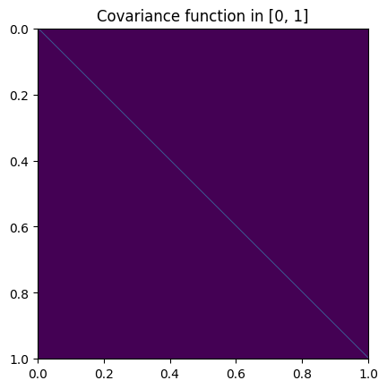
\[\begin{split}K(x, x')= \begin{cases} \sigma^2, \quad x = x' \\ 0, \quad x \neq x'\\ \end{cases}\end{split}\]where \(\sigma^2\) is the variance.
Heatmap plot of the covariance function:
from skfda.misc.covariances import WhiteNoise
import matplotlib.pyplot as plt

WhiteNoise().heatmap(limits=(0, 1))
plt.show()
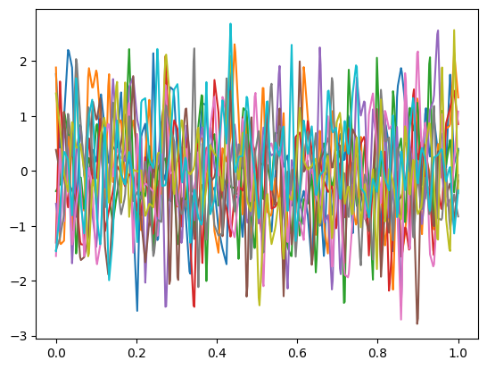
Example of Gaussian process trajectories using this covariance:
from skfda.misc.covariances import WhiteNoise
from skfda.datasets import make_gaussian_process
import matplotlib.pyplot as plt

gp = make_gaussian_process(
        n_samples=10, cov=WhiteNoise(), random_state=0)
gp.plot()
plt.show()
Default representation in a Jupyter notebook:
from skfda.misc.covariances import WhiteNoise

WhiteNoise()
\[K(x, x')= \begin{cases} \sigma^2, \quad x = x' \\0, \quad x \neq x'\\ \end{cases} \\\text{where:}\begin{aligned}\qquad\sigma^2 &= 1 \\\end{aligned}\]Methods
heatmap([limits])Return a heatmap plot of the covariance function.
Obtain corresponding scikit-learn kernel type.
- Parameters:
variance (float)