Brownian#
- class skfda.misc.covariances.Brownian(*, variance=1, origin=0)[source]#
Brownian covariance function.
The covariance function is
\[K(x, x') = \sigma^2 \frac{|x - \mathcal{O}| + |x' - \mathcal{O}| - |x - x'|}{2}\]where \(\sigma^2\) is the variance at distance 1 from \(\mathcal{O}\) and \(\mathcal{O}\) is the origin point. If \(\mathcal{O} = 0\) (the default) and we only consider positive values, the formula can be simplified as
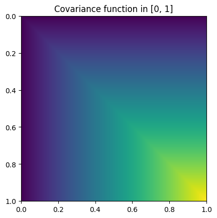
\[K(x, y) = \sigma^2 \min(x, y).\]Heatmap plot of the covariance function:
from skfda.misc.covariances import Brownian
import matplotlib.pyplot as plt

Brownian().heatmap(limits=(0, 1))
plt.show()
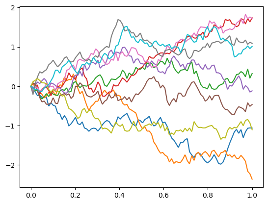
Example of Gaussian process trajectories using this covariance:
from skfda.misc.covariances import Brownian
from skfda.datasets import make_gaussian_process
import matplotlib.pyplot as plt

gp = make_gaussian_process(
        n_samples=10, cov=Brownian(), random_state=0)
gp.plot()
plt.show()
Default representation in a Jupyter notebook:
from skfda.misc.covariances import Brownian

Brownian()
\[K(x, x') = \sigma^2 \frac{|x - \mathcal{O}| + |x' - \mathcal{O}| - |x - x'|}{2} \\\text{where:}\begin{aligned}\qquad\sigma^2 &= 1 \\\mathcal{O} &= 0 \\\end{aligned}\]Methods
heatmap([limits])Return a heatmap plot of the covariance function.
Convert it to a sklearn kernel, if there is one.