Creating a new basis

Shows how to add new bases for FDataBasis by creating subclasses.

# Author: Carlos Ramos Carreño
# License: MIT

import matplotlib.pyplot as plt
import numpy as np

In this example, we want to showcase how it is possible to make new functional bases compatible with FDataBasis, by subclassing the Basis class.

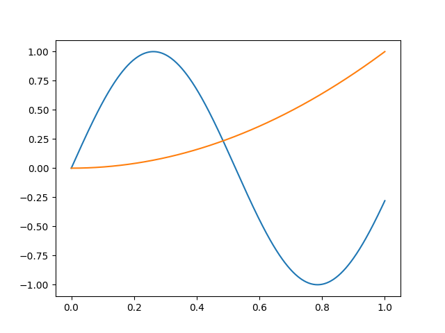
Suppose that we already know that our data belongs to (or can be reasonably approximated in) the functional space spanned by the basis \(\{f(t) = \sin(6t), g(t) = t^2\}\). We can define these two functions in Python as follows (remember than the input and output are both NumPy arrays).

def f(t):
    return np.sin(6 * t)


def g(t):
    return t**2

Lets now define the functional basis. We create a subclass of Basis containing the definition of our desired basis. We need to overload the __init__ method in order to add the necessary parameters for the creation of the basis. Basis requires both the domain range and the number of elements in the basis in order to work. As this particular basis has fixed size, we only expose the domain_range parameter in the constructor, but we still pass the fixed size to the parent class constructor.

It is also necessary to override the protected _evaluate method, that defines the evaluation of the basis elements.

from skfda.representation.basis import Basis


class MyBasis(Basis):
    """Basis of f and g."""

    def __init__(
        self,
        *,
        domain_range=None,
    ):
        super().__init__(domain_range=domain_range, n_basis=2)

    def _evaluate(
        self,
        eval_points,
    ):
        return np.vstack([
            f(eval_points),
            g(eval_points),
        ])

We can now create an instance of this basis and plot it.

basis = MyBasis()
basis.plot()
plt.show()

This simple definition already allows to represent functions and work with them, but it does not allow advanced functionality such as taking derivatives (because it does not know how to derive the basis elements!). In order to add support for that we would need to override the appropriate methods (in this case, _derivative_basis_and_coefs).

In this particular case, we are not interested in the derivatives, only in correct representation and evaluation. We can now test the conversion from FDataGrid to FDataBasis for elements in this space.

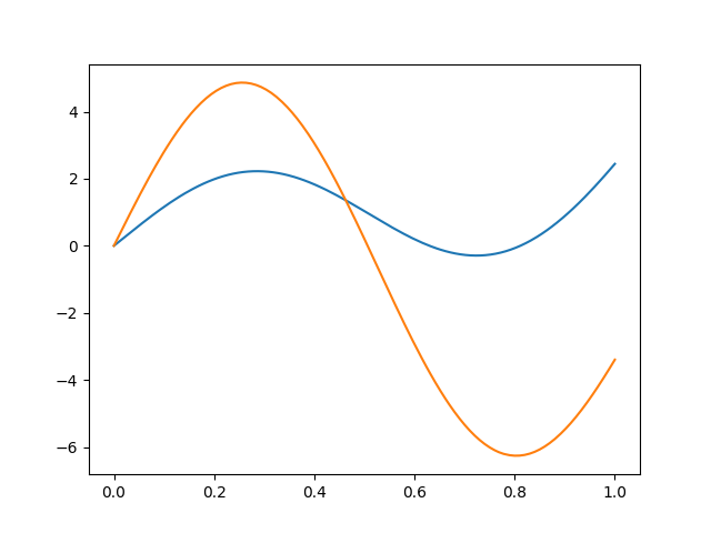
We first define a (discretized) function in the space spanned by \(f\) and \(g\).

from skfda.representation import FDataGrid

t = np.linspace(0, 1, 100)
data_matrix = [
    2 * f(t) + 3 * g(t),
    5 * f(t) - 2 * g(t),
]

X = FDataGrid(data_matrix, grid_points=t)
X.plot()
plt.show()

We can now convert it to our basis, and visually check that the representation is exact.

X_basis = X.to_basis(basis)
X_basis.plot()
plt.show()

If we inspect the coefficients, we can finally guarantee that they are the ones used in the initial definition.

X_basis.coefficients

array([[ 2.,  3.],
       [ 5., -2.]])

Lets consider a more complex example. Suppose that we want to create a basis adapted to the data using the principal components. One approach could be creating a basis that computes FPCA and uses the components obtained. Note that equality should be overriden as it is no longer true that two instances of this basis with the same domain and number of elements are equal.

from skfda.preprocessing.dim_reduction import FPCA


class FPCABasis(Basis):
    """Basis of principal components."""

    def __init__(
        self,
        *,
        X,
        n_basis=1,
    ):
        super().__init__(domain_range=X.domain_range, n_basis=n_basis)

        self._fpca = FPCA(n_components=n_basis)
        self._fpca.fit(X)

    def _evaluate(
        self,
        eval_points,
    ):
        return self._fpca.components_(eval_points)

    def __eq__(self, other):
        return (
            super().__eq__(self, other)
            and self._fpca.components_ == other._fpca.components_
        )

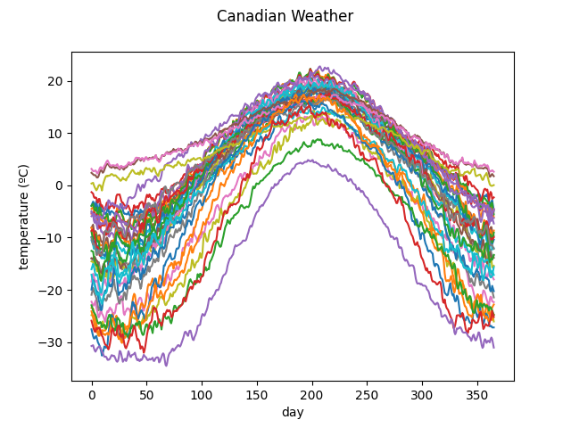
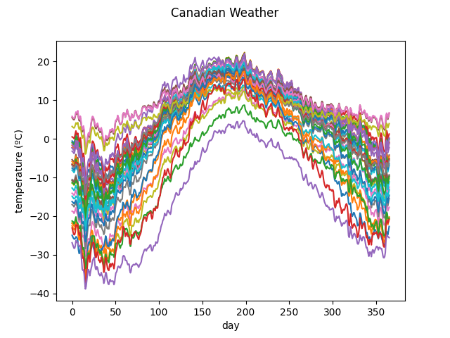
We now load the temperatures from the Canadian Weather dataset and plot them.

from skfda.datasets import fetch_weather

X, y = fetch_weather(return_X_y=True)
X = X.coordinates[0]
X.plot()
plt.show()

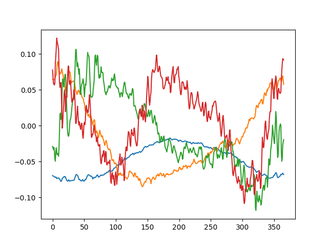
We construct the new FPCA basis from the data, using 4 basis elements. We plot the basis elements, which correspond with the first 4 principal components of the data.

basis = FPCABasis(X=X, n_basis=4)
basis.plot()
plt.show()

We can now represent the original data using this basis.

X_basis = X.to_basis(basis)
X_basis.plot()
plt.show()