Functional Linear Regression with multivariate covariates.

This example explores the use of the linear regression with multivariate (scalar) covariates and functional response.

# Author: Rafael Hidalgo Alejo
# License: MIT

import numpy as np
import pandas as pd
from sklearn.preprocessing import OneHotEncoder

import skfda
from skfda.ml.regression import LinearRegression
from skfda.representation.basis import FDataBasis, FourierBasis

In this example, we will demonstrate the use of the Linear Regression with functional response and multivariate covariates using the weather dataset. It is possible to divide the weather stations into four groups: Atlantic, Pacific, Continental and Artic. There are a total of 35 stations in this dataset.

X_weather, y_weather = skfda.datasets.fetch_weather(
    return_X_y=True, as_frame=True,
)
fd = X_weather.iloc[:, 0].values

The main goal is knowing about the effect of stations’ geographic location on the shape of the temperature curves. So we will have a model with a functional response, the temperature curve, and five covariates. The first one is the intercept (all entries equal to 1) and it shows the contribution of the Canadian mean temperature. The remaining covariates use one-hot encoding, with 1 if that weather station is in the corresponding climate zone and 0 otherwise.

# We first create the one-hot encoding of the climates.

enc = OneHotEncoder(handle_unknown='ignore')
enc.fit([['Atlantic'], ['Continental'], ['Pacific']])
X = np.array(y_weather).reshape(-1, 1)
X = enc.transform(X).toarray()

Then, we construct a dataframe with each covariate in a different column and the temperature curves (responses).

X_df = pd.DataFrame(X)

y_basis = FourierBasis(n_basis=65)
y_fd = fd.coordinates[0].to_basis(y_basis)

An intercept term is incorporated. All functional coefficients will have the same basis as the response.

funct_reg = LinearRegression(fit_intercept=True)
funct_reg.fit(X_df, y_fd)

LinearRegression()

In a Jupyter environment, please rerun this cell to show the HTML representation or trust the notebook.
On GitHub, the HTML representation is unable to render, please try loading this page with nbviewer.org.

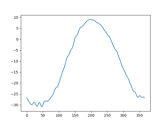
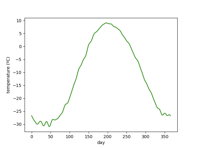
The regression coefficients are shown below. The first one is the intercept coefficient, corresponding to Canadian mean temperature.

funct_reg.intercept_.plot()
funct_reg.coef_[0].plot()
funct_reg.coef_[1].plot()
funct_reg.coef_[2].plot()

• 
• 
• 
• 

<Figure size 640x480 with 1 Axes>

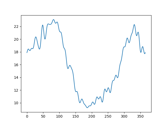
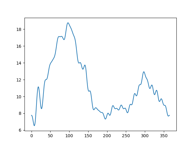
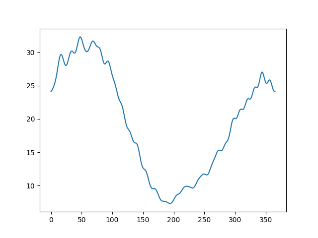
Finally, it is shown a panel with the prediction for all climate zones.

predictions = []

predictions.append(funct_reg.predict([[0, 1, 0, 0]])[0])
predictions.append(funct_reg.predict([[0, 0, 1, 0]])[0])
predictions.append(funct_reg.predict([[0, 0, 0, 1]])[0])

predictions_conc = FDataBasis.concatenate(*predictions)

predictions_conc.argument_names = ('day',)
predictions_conc.coordinate_names = ('temperature (ºC)',)

predictions_conc.plot()

<Figure size 640x480 with 1 Axes>