Depth based classification

This example shows the use of the depth based classification methods applied to the Berkeley Growth Study data. An attempt to show the differences and similarities between MaximumDepthClassifier, DDClassifier, and DDGClassifier is made.

# Author: Pedro Martín Rodríguez-Ponga Eyriès
# License: MIT

# sphinx_gallery_thumbnail_number = 5

import matplotlib.pyplot as plt
import numpy as np
from matplotlib.colors import ListedColormap
from sklearn.model_selection import train_test_split
from sklearn.neighbors import KNeighborsClassifier
from sklearn.neural_network import MLPClassifier

from skfda import datasets
from skfda.exploratory.depth import ModifiedBandDepth
from skfda.exploratory.visualization import DDPlot
from skfda.ml.classification import (
    DDClassifier,
    DDGClassifier,
    MaximumDepthClassifier,
)
from skfda.preprocessing.feature_construction import PerClassTransformer

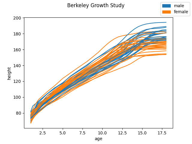
The Berkeley Growth Study data contains the heights of 39 boys and 54 girls from age 1 to 18 and the ages at which they were collected. Males are assigned the numeric value 0 while females are assigned a 1. In our comparison of the different methods, we will try to learn the sex of a person by using its growth curve.

X, y = datasets.fetch_growth(return_X_y=True, as_frame=True)
X = X.iloc[:, 0].values
categories = y.values.categories
y = y.values.codes

As in many ML algorithms, we split the dataset into train and test. In this graph, we can see the training dataset. These growth curves will be used to train the model. Hence, the predictions will be data-driven.

X_train, X_test, y_train, y_test = train_test_split(
    X,
    y,
    test_size=0.5,
    stratify=y,
    random_state=0,
)

# Plot samples grouped by sex
X_train.plot(group=y_train, group_names=categories).show()

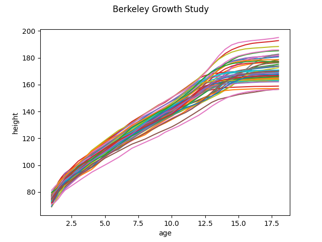
Below are the growth graphs of those individuals that we would like to classify. Some of them will be male and some female.

X_test.plot().show()

As said above, we are trying to compare three different methods: MaximumDepthClassifier, DDClassifier, and DDGClassifier. They all use a depth which in our example is ModifiedBandDepth for consistency. With this depth we can create a DDPlot.

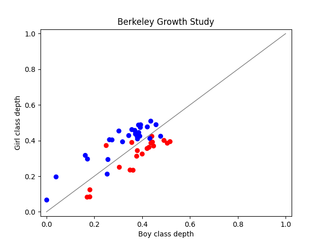
In a DDPlot, a growth curve is mapped to \([0,1]\times[0,1]\) where the first coordinate corresponds to the depth in the class of all boys and the second to that of all girls. Note that the dots will be blue if the true sex is female and red otherwise.

Below we can see how a DDPlot is used to classify with MaximumDepthClassifier. In this case it is quite straighforward, a person is classified to the class where it is deeper. This means that if a point is above the diagonal it is a girl and otherwise it is a boy.

clf = MaximumDepthClassifier(depth_method=ModifiedBandDepth())
clf.fit(X_train, y_train)
print(clf.predict(X_test))
print('The score is {0:2.2%}'.format(clf.score(X_test, y_test)))

fig, ax = plt.subplots()

cmap_bold = ListedColormap(['#FF0000', '#0000FF'])

index = y_train.astype(bool)
DDPlot(
    fdata=X_test,
    dist1=X_train[np.invert(index)],
    dist2=X_train[index],
    depth_method=ModifiedBandDepth(),
    axes=ax,
    c=y_test,
    cmap_bold=cmap_bold,
    x_label="Boy class depth",
    y_label="Girl class depth",
).plot().show()

[0 0 0 0 0 0 1 1 1 1 0 1 0 0 0 1 0 1 0 1 1 1 0 1 1 0 0 0 1 1 1 1 1 0 1 1 0
 0 1 1 1 0 0 1 1 1 1]
The score is 89.36%

We can see that we have used the classification predictions to compute the score (obtained by comparing to the real known sex). This will also be done for the rest of the classifiers.

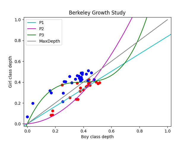
Next we use DDClassifier with polynomes of degrees one, two, and three. Here, if a point in the DDPlot is above the polynome, the classifier will predict that it is a girl and otherwise, a boy.

clf1 = DDClassifier(degree=1, depth_method=ModifiedBandDepth())
clf1.fit(X_train, y_train)
print(clf1.predict(X_test))
print('The score is {0:2.2%}'.format(clf1.score(X_test, y_test)))

[0 0 1 0 1 1 1 1 1 1 1 1 1 0 0 1 0 1 0 1 1 1 1 1 1 0 0 1 1 1 1 1 1 1 1 1 0
 0 1 1 1 0 0 1 1 1 1]
The score is 80.85%

clf2 = DDClassifier(degree=2, depth_method=ModifiedBandDepth())
clf2.fit(X_train, y_train)
print(clf2.predict(X_test))
print('The score is {0:2.2%}'.format(clf2.score(X_test, y_test)))

[0 0 1 1 1 1 1 1 1 1 1 1 1 1 0 1 0 1 1 1 1 1 1 1 1 0 1 1 1 1 1 1 1 0 1 1 1
 1 1 1 1 0 1 1 1 1 1]
The score is 68.09%

clf3 = DDClassifier(degree=3, depth_method=ModifiedBandDepth())
clf3.fit(X_train, y_train)
print(clf3.predict(X_test))
print('The score is {0:2.2%}'.format(clf3.score(X_test, y_test)))

[0 0 1 0 0 1 1 1 1 1 0 1 0 0 0 1 0 1 0 0 1 1 0 1 0 0 0 0 0 1 1 0 1 1 1 1 0
 0 1 1 1 0 0 1 1 0 1]
The score is 89.36%

fig, ax = plt.subplots()


def _plot_boundaries(axis):
    margin = 0.025
    ts = np.linspace(- margin, 1 + margin, 100)
    pol1 = axis.plot(
        ts,
        np.polyval(clf1.poly_, ts),
        'c',
        label="Polynomial",
    )[0]
    pol2 = axis.plot(
        ts,
        np.polyval(clf2.poly_, ts),
        'm',
        label="Polynomial",
    )[0]
    pol3 = axis.plot(
        ts,
        np.polyval(clf3.poly_, ts),
        'g',
        label="Polynomial",
    )[0]
    max_depth = axis.plot(
        [0, 1],
        color="gray",
    )[0]

    axis.legend([pol1, pol2, pol3, max_depth], ['P1', 'P2', 'P3', 'MaxDepth'])


_plot_boundaries(ax)

DDPlot(
    fdata=X_test,
    dist1=X_train[np.invert(index)],
    dist2=X_train[index],
    depth_method=ModifiedBandDepth(),
    axes=ax,
    c=y_test,
    cmap_bold=cmap_bold,
    x_label="Boy class depth",
    y_label="Girl class depth",
).plot().show()

DDClassifier used with KNeighborsClassifier.

clf = DDGClassifier(
    depth_method=ModifiedBandDepth(),
    multivariate_classifier=KNeighborsClassifier(n_neighbors=5),
)
clf.fit(X_train, y_train)
print(clf.predict(X_test))
print('The score is {0:2.2%}'.format(clf.score(X_test, y_test)))

[1 0 1 1 0 1 1 1 1 1 0 1 0 0 0 1 0 1 0 1 1 1 0 1 1 0 1 0 1 1 1 1 1 0 1 1 0
 0 1 1 1 1 0 1 1 1 1]
The score is 85.11%

The other elements of the graph are the decision boundaries:

Boundary	Classifier
MaxDepth	MaximumDepthClassifier
P1	DDClassifier with degree 1
P2	DDClassifier with degree 2
P3	DDClassifier with degree 3
NearestClass	DDGClassifier with nearest neighbors

pct = PerClassTransformer(ModifiedBandDepth(), array_output=True)
X_train_trans = pct.fit_transform(X_train, y_train)
X_train_trans = X_train_trans.reshape(len(categories), X_train.shape[0]).T

clf = KNeighborsClassifier(n_neighbors=5)
clf.fit(X_train_trans, y_train)

h = 0.01  # step size in the mesh

# Create color maps
cmap_light = ListedColormap(['#FFAAAA', '#AAAAFF'])

# Plot the decision boundary. For that, we will assign a color to each
# point in the mesh [x_min, x_max]x[y_min, y_max].
x_min, x_max = X_train_trans[:, 0].min() - 1, X_train_trans[:, 0].max() + 1
y_min, y_max = X_train_trans[:, 1].min() - 1, X_train_trans[:, 1].max() + 1
xx, yy = np.meshgrid(
    np.arange(x_min, x_max, h),
    np.arange(y_min, y_max, h),
)
Z = clf.predict(np.c_[xx.ravel(), yy.ravel()])

# Put the result into a color plot
Z = Z.reshape(xx.shape)

fig, ax = plt.subplots()
ax.pcolormesh(xx, yy, Z, cmap=cmap_light, shading='auto')

_plot_boundaries(ax)
DDPlot(
    fdata=X_test,
    dist1=X_train[np.invert(index)],
    dist2=X_train[index],
    depth_method=ModifiedBandDepth(),
    axes=ax,
    c=y_test,
    cmap_bold=cmap_bold,
    x_label="Boy class depth",
    y_label="Girl class depth",
).plot().show()

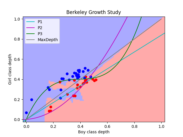
In the above graph, we can see the obtained classifiers from the train set. The dots are all part of the test set and have their real color so, for example, if they are blue it means that the true sex is female. One can see that none of the built classifiers is perfect.

Next, we will use DDGClassifier together with a neural network: MLPClassifier.

clf = DDGClassifier(
    depth_method=ModifiedBandDepth(),
    multivariate_classifier=MLPClassifier(
        solver='lbfgs',
        alpha=1e-5,
        hidden_layer_sizes=(6, 2),
        random_state=1,
    ),
)
clf.fit(X_train, y_train)
print(clf.predict(X_test))
print('The score is {0:2.2%}'.format(clf.score(X_test, y_test)))

[0 0 0 0 0 0 1 1 1 1 0 1 0 0 0 1 0 1 0 1 1 1 0 1 1 0 0 0 1 1 1 1 1 0 1 1 0
 0 1 1 1 0 0 1 1 1 1]
The score is 89.36%

clf1 = KNeighborsClassifier(n_neighbors=5)
clf2 = MLPClassifier(
    solver='lbfgs',
    alpha=1e-5,
    hidden_layer_sizes=(6, 2),
    random_state=1,
)
clf1.fit(X_train_trans, y_train)
clf2.fit(X_train_trans, y_train)

Z1 = clf1.predict(np.c_[xx.ravel(), yy.ravel()])
Z2 = clf2.predict(np.c_[xx.ravel(), yy.ravel()])

Z1 = Z1.reshape(xx.shape)
Z2 = Z2.reshape(xx.shape)

fig, axs = plt.subplots(1, 2, sharex=True, sharey=True)

axs[0].pcolormesh(xx, yy, Z1, cmap=cmap_light, shading='auto')
axs[1].pcolormesh(xx, yy, Z2, cmap=cmap_light, shading='auto')

DDPlot(
    fdata=X_test,
    dist1=X_train[np.invert(index)],
    dist2=X_train[index],
    depth_method=ModifiedBandDepth(),
    axes=axs[0],
    c=y_test,
    cmap_bold=cmap_bold,
    x_label="Boy class depth",
    y_label="Girl class depth",
).plot().show()
DDPlot(
    fdata=X_test,
    dist1=X_train[np.invert(index)],
    dist2=X_train[index],
    depth_method=ModifiedBandDepth(),
    axes=axs[1],
    c=y_test,
    cmap_bold=cmap_bold,
    x_label="Boy class depth",
    y_label="Girl class depth",
).plot().show()

for axis in axs:
    axis.label_outer()

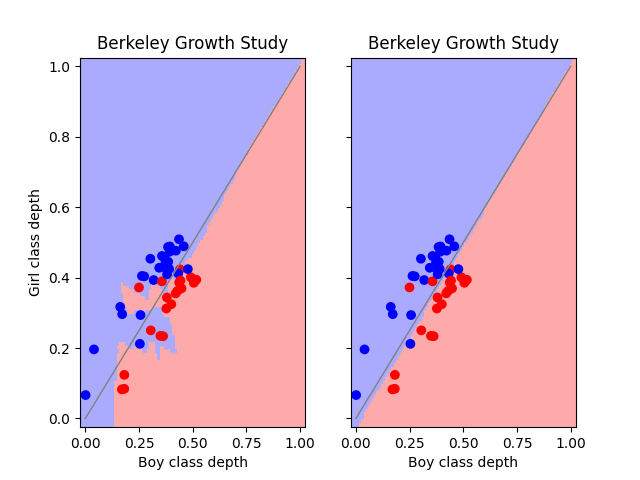
We can compare the behavior of two DDGClassifier based classifiers. The one on the left corresponds to nearest neighbors and the one on the right to a neural network. Interestingly, the neural network almost coincides with MaximumDepthClassifier.