Surface Boxplot

Shows the use of the surface boxplot, which is a generalization of the functional boxplot for FDataGrid whose domain dimension is 2.

# Author: Amanda Hernando Bernabé
# License: MIT

# sphinx_gallery_thumbnail_number = 3

from skfda import FDataGrid
from skfda.datasets import make_gaussian_process
from skfda.exploratory.visualization import SurfaceBoxplot, Boxplot

import matplotlib.pyplot as plt
import numpy as np

In order to instantiate a SurfaceBoxplot, a functional data object with bidimensional domain must be generated. In this example, a FDataGrid representing a function \(f : \mathbb{R}^2\longmapsto\mathbb{R}\) is constructed, using as an example a Brownian process extruded into another dimension.

The values of the Brownian process are generated using make_gaussian_process(), Those functions return FDataGrid objects whose data_matrix store the values needed.

n_samples = 10
n_features = 10

fd = make_gaussian_process(n_samples=n_samples, n_features=n_features,
                           random_state=1)
fd.dataset_name = "Brownian process"

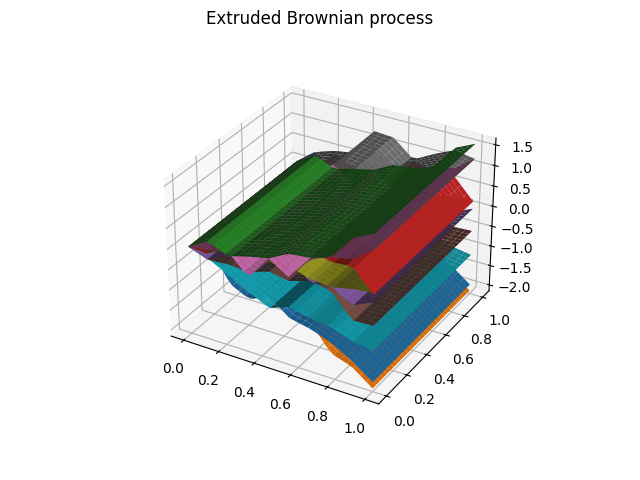
After, those values generated for one dimension on the domain are extruded along another dimension, obtaining a three-dimensional matrix or cube (two-dimensional domain and one-dimensional image).

cube = np.repeat(fd.data_matrix, n_features).reshape(
    (n_samples, n_features, n_features))

We can plot now the extruded trajectories.

fd_2 = FDataGrid(data_matrix=cube,
                 grid_points=np.tile(fd.grid_points, (2, 1)),
                 dataset_name="Extruded Brownian process")

fd_2.plot()

<Figure size 640x480 with 1 Axes>

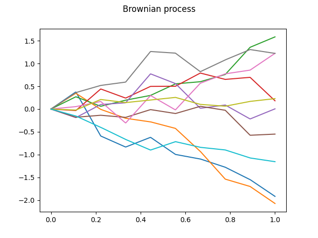
Since matplotlib was initially designed with only two-dimensional plotting in mind, the three-dimensional plotting utilities were built on top of matplotlib’s two-dimensional display, and the result is a convenient (if somewhat limited) set of tools for three-dimensional data visualization as we can observe.

For this reason, the profiles of the surfaces, which are contained in the first two generated functional data objects, are plotted below, to help to visualize the data.

fd.plot()

<Figure size 640x480 with 1 Axes>

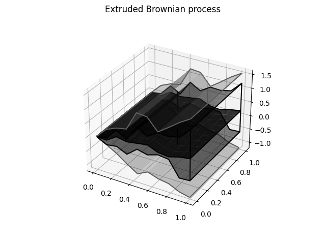
To terminate the example, the instantiation of the SurfaceBoxplot object is made, showing the surface boxplot which corresponds to our FDataGrid

surfaceBoxplot = SurfaceBoxplot(fd_2)
surfaceBoxplot.plot()

<Figure size 640x480 with 1 Axes>

The surface boxplot contains the median, the central envelope and the outlying envelope plotted from darker to lighter colors, although they can be customized.

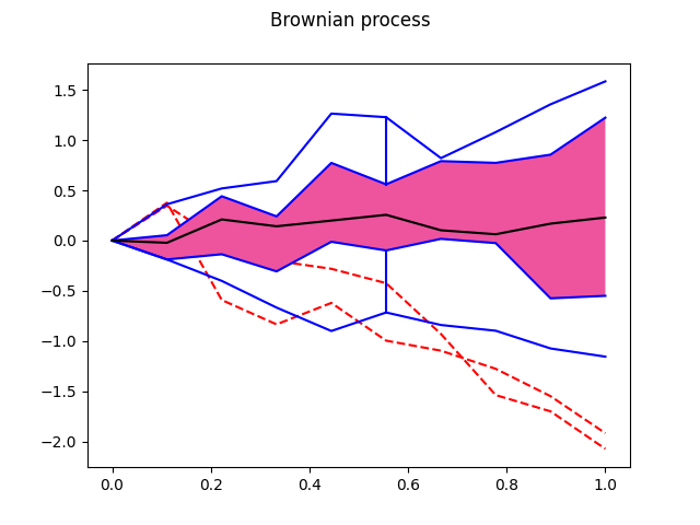
Analogous to the procedure followed before of plotting the three-dimensional data and their correponding profiles, we can obtain also the functional boxplot for one-dimensional data with the Boxplot passing as arguments the first FdataGrid object. The profile of the surface boxplot is obtained.

boxplot1 = Boxplot(fd)
boxplot1.plot()

<Figure size 640x480 with 1 Axes>