Spectrometric data: derivatives, regression, and variable selection

Shows the use of derivatives, functional regression and variable selection for functional data.

# License: MIT

# sphinx_gallery_thumbnail_number = 4

import matplotlib.pyplot as plt
import sklearn.linear_model
from sklearn.metrics import r2_score
from sklearn.model_selection import train_test_split
from sklearn.pipeline import Pipeline
from sklearn.tree import DecisionTreeRegressor, plot_tree

from skfda.datasets import fetch_tecator
from skfda.ml.regression import LinearRegression
from skfda.preprocessing.dim_reduction.variable_selection.maxima_hunting import (
    MaximaHunting,
    RelativeLocalMaximaSelector,
)
from skfda.representation.basis import BSplineBasis

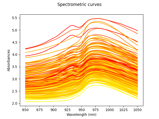
This example uses the Tecator dataset[1] in order to illustrate the problems of functional regression and functional variable selection. This dataset contains the spectra of absorbances of several pieces of finely chopped meat, as well as the percent of its content in water, fat and protein.

This is one of the examples presented in the ICTAI conference[2].

We will first load the Tecator data, keeping only the fat content target, and plot it.

X, y = fetch_tecator(return_X_y=True)
y = y[:, 0]

X.plot(gradient_criteria=y)
plt.show()

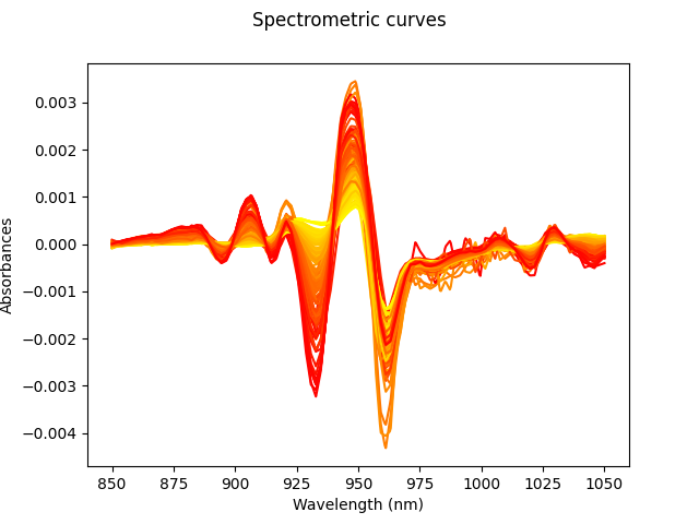
For spectrometric data, the relevant information of the curves can often be found in the derivatives[3]. Thus, we compute numerically the second derivative and plot it.

X_der = X.derivative(order=2)
X_der.plot(gradient_criteria=y)
plt.show()

We first apply a simple linear regression model to compute a baseline for our regression predictions. In order to compute functional linear regression we first convert the data to a basis expansion.

basis = BSplineBasis(
    n_basis=10,
)
X_der_basis = X_der.to_basis(basis)

We split the data in train and test, and compute the regression score using the linear regression model.

X_train, X_test, y_train, y_test = train_test_split(
    X_der_basis,
    y,
    random_state=0,
)

regressor = LinearRegression()
regressor.fit(X_train, y_train)
y_pred = regressor.predict(X_test)
score = r2_score(y_test, y_pred)
print(score)

0.9505439228770038

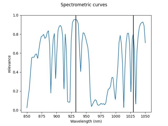
We now will take a different approach. It is possible to note from the plot of the derivatives that most information necessary for regression can be found at some particular “impact” points. Thus, we now apply a functional variable selection method to detect those points and use them with a multivariate classifier. The variable selection method that we employ here is maxima hunting[4], a filter method that computes a relevance score for each point of the curve and selects all the local maxima.

var_sel = MaximaHunting(
    local_maxima_selector=RelativeLocalMaximaSelector(max_points=2),
)
X_mv = var_sel.fit_transform(X_der, y)

print(var_sel.indexes_)

[41 89]

We can visualize the relevance function and the selected points.

var_sel.dependence_.plot()
for p in var_sel.indexes_:
    plt.axvline(X_der.grid_points[0][p], color="black")
plt.show()

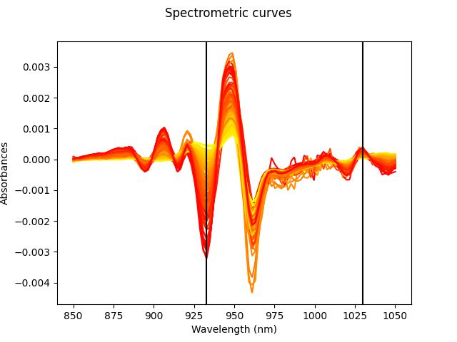
We also can visualize the selected points on the curves.

X_der.plot(gradient_criteria=y)
for p in var_sel.indexes_:
    plt.axvline(X_der.grid_points[0][p], color="black")
plt.show()

We split the data again (using the same seed), but this time without the basis expansion.

X_train, X_test, y_train, y_test = train_test_split(
    X_der,
    y,
    random_state=0,
)

We now make a pipeline with the variable selection and a multivariate linear regression method for comparison.

pipeline = Pipeline([
    ("variable_selection", var_sel),
    ("classifier", sklearn.linear_model.LinearRegression()),
])
pipeline.fit(X_train, y_train)
y_predicted = pipeline.predict(X_test)
score = r2_score(y_test, y_predicted)
print(score)

0.8959181661493842

We can use a tree regressor instead to improve both the score and the interpretability.

pipeline = Pipeline([
    ("variable_selection", var_sel),
    ("classifier", DecisionTreeRegressor(max_depth=3)),
])
pipeline.fit(X_train, y_train)
y_predicted = pipeline.predict(X_test)
score = r2_score(y_test, y_predicted)
print(score)

0.9417361615246084

We can plot the final version of the tree to explain every prediction.

fig, ax = plt.subplots(figsize=(10, 10))
plot_tree(pipeline.named_steps["classifier"], precision=6, filled=True, ax=ax)
plt.show()

References

[1]

\relax Claus. Borggaard and Hans Henrik. Thodberg. Optimal minimal neural interpretation of spectra. Analytical Chemistry, 64(5):545–551, March 1992. URL: https://doi.org/10.1021/ac00029a018 (visited on 2018-12-09), doi:10.1021/ac00029a018.

[2]

Carlos Ramos-Carreño, José Luis Torrecilla, Yujian Hong, and Alberto Suárez. scikit-fda: Computational tools for machine learning with functional data. In 2022 IEEE 34th International Conference on Tools with Artificial Intelligence (ICTAI), 213–218. October 2022. doi:10.1109/ICTAI56018.2022.00038.

[3]

Frédéric Ferraty and Philippe Vieu. Computational Issues, pages 99–108. Springer Series in Statistics. Springer-Verlag, New York, 2006. URL: https://www.springer.com/gp/book/9780387303697 (visited on 2019-09-10).

[4]

José Ramón Berrendero, Antonio Cuevas, and José Luis Torrecilla. Variable selection in functional data classification: a maxima-hunting proposal. Statistica Sinica, 26(2):619–638, 2016. URL: http://www3.stat.sinica.edu.tw/statistica/J26N2/J26N210/J26N210.html (visited on 2019-09-02), doi:10.5705/ss.202014.0014.