Note
Go to the end to download the full example code. or to run this example in your browser via Binder
Interpolation#
This example shows the types of interpolation used in the evaluation of FDataGrids.
# Author: Pablo Marcos Manchón
# License: MIT

# sphinx_gallery_thumbnail_number = 3

import matplotlib.pyplot as plt
import numpy as np
from mpl_toolkits.mplot3d import axes3d

import skfda
from skfda.representation.interpolation import SplineInterpolation
The FDataGrid class is used for datasets
containing discretized functions. For the evaluation between the points of
discretization, or sample points, is necessary to interpolate.
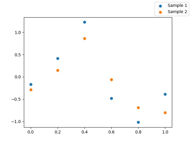
We will construct an example dataset with two curves with 6 points of discretization.
fd = skfda.datasets.make_sinusoidal_process(
    n_samples=2,
    n_features=6,
    random_state=1,
)
fig = fd.scatter()
fig.legend(["Sample 1", "Sample 2"])
plt.show()
By default it is used linear interpolation, which is one of the simplest methods of interpolation and therefore one of the least computationally expensive, but has the disadvantage that the interpolant is not differentiable at the points of discretization.
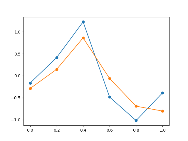
The interpolation method of the FDataGrid could be changed setting the
attribute interpolation. Once we have set an interpolation it is used for
the evaluation of the object.
Polynomial spline interpolation could be performed using the interpolation
SplineInterpolation. In the
following example a cubic interpolation is set.
fd.interpolation = SplineInterpolation(interpolation_order=3)
fig = fd.plot()
fd.scatter(fig=fig)
plt.show()
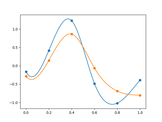
Sometimes our samples are required to be monotone, in these cases it is
possible to use monotone cubic interpolation with the attribute
monotone. A piecewise cubic hermite interpolating polynomial (PCHIP)
will be used.
fd = fd[1]

fd_monotone = fd.copy(data_matrix=np.sort(fd.data_matrix, axis=1))


fig = fd_monotone.plot(linestyle='--', label="cubic")


fd_monotone.interpolation = SplineInterpolation(
    interpolation_order=3,
    monotone=True,
)
fd_monotone.plot(fig=fig, label="PCHIP")

fd_monotone.scatter(fig=fig, c='C1')
fig.legend()
plt.show()
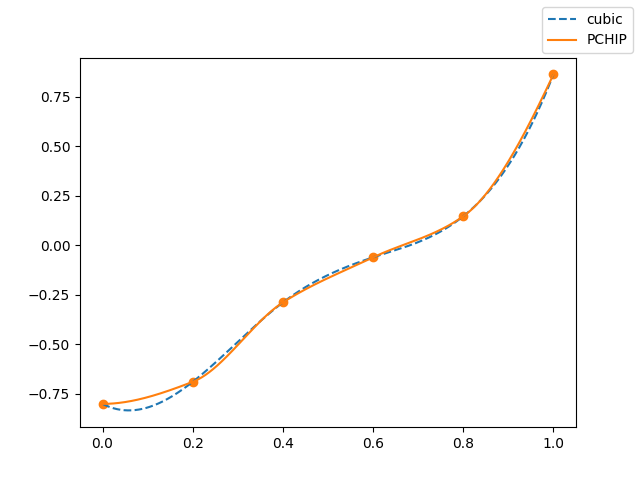
All the interpolations will work regardless of the dimension of the image, but depending on the domain dimension some methods will not be available.
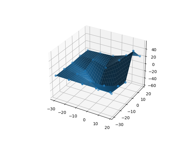
For the next examples it is constructed a surface, \(x_i: \mathbb{R}^2 \longmapsto \mathbb{R}\). By default, as in unidimensional samples, it is used linear interpolation.
X, Y, Z = axes3d.get_test_data(1.2)
data_matrix = [Z.T]
grid_points = [X[0, :], Y[:, 0]]


fd = skfda.FDataGrid(data_matrix, grid_points)

fig = fd.plot()
fd.scatter(fig=fig)
plt.show()
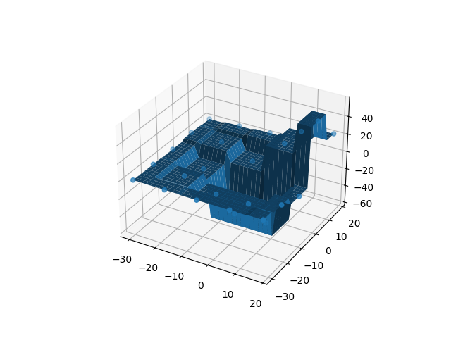
In the following figure it is shown the result of the constant interpolation applied to the surface.
fd.interpolation = SplineInterpolation(interpolation_order=0)

fig = fd.plot()
fd.scatter(fig=fig)
plt.show()
Total running time of the script: (0 minutes 0.431 seconds)