Note
Go to the end to download the full example code. or to run this example in your browser via Binder
Landmark registration#
This example shows the basic usage of the landmark registration.
# Author: Pablo Marcos Manchón
# License: MIT

import matplotlib.pyplot as plt
import numpy as np

import skfda
The simplest curve alignment procedure is landmark registration. This method only takes into account a discrete ammount of features of the curves which will be registered.
A landmark or a feature of a curve is some characteristic that one can associate with a specific argument value t. These are typically maxima, minima, or zero crossings of curves, and may be identified at the level of some derivatives as well as at the level of the curves themselves. We align the curves by transforming t for each curve so that landmark locations are the same for all curves ( [RaSi2005] , [RaHoGr2009] ).
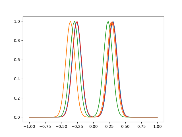
We will use a dataset synthetically generated by
make_multimodal_samples(), which in this case will
be used to generate bimodal curves.
fd = skfda.datasets.make_multimodal_samples(
    n_samples=4,
    n_modes=2,
    std=0.002,
    mode_std=0.005,
    random_state=1,
)
fd.plot()
<Figure size 640x480 with 1 Axes>
For this type of alignment we need to know in advance the location of the
landmarks of each of the samples, in our case it will correspond to the two
maximum points of each sample.
Because our dataset has been generated synthetically we can obtain the value
of the landmarks using the function
make_multimodal_landmarks(), which is used by
make_multimodal_samples() to set the location of the
modes.
In general it will be necessary to use numerical or other methods to determine the location of the landmarks.
landmarks = skfda.datasets.make_multimodal_landmarks(
    n_samples=4,
    n_modes=2,
    std=0.002,
    random_state=1,
).squeeze()

print(landmarks)
[[-0.2606904   0.30597475]
 [-0.35695389  0.28534872]
 [-0.29463113  0.23040539]
 [-0.25530298  0.29929113]]
The transformation will not be linear, and will be the result of applying a warping function to the time of our curves.
After the identification of the landmarks asociated with the features of
each of our curves we can construct the warping function with the function
landmark_elastic_registration_warping().
Let \(h_i\) be the warping function corresponding with the curve \(i\), \(t_{ij}\) the time where the curve \(i\) has their feature \(j\) and \(t^*_j\) the new location of the feature \(j\). The warping functions will transform the new time in the original time of the curve, i.e., \(h_i(t^*_j) = t_{ij}\). These functions will be defined between landmarks using monotone cubic interpolation (see the example of interpolation for more details).
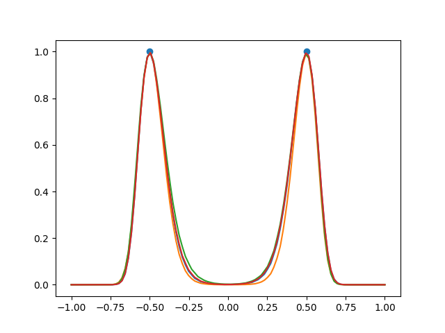
In this case we will place the landmarks at -0.5 and 0.5.
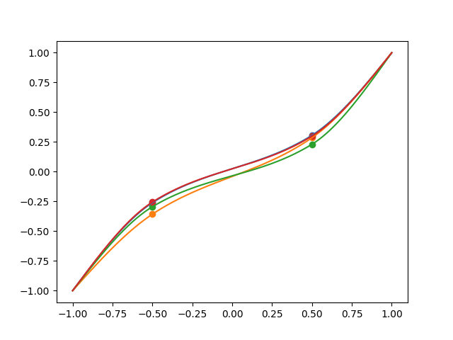
Once we have the warping functions, the registered curves can be obtained using function composition. Let \(x_i\) a curve, we can obtain the corresponding registered curve as \(x^*_i(t) = x_i(h_i(t))\).
<matplotlib.collections.PathCollection object at 0x79b41ee746d0>
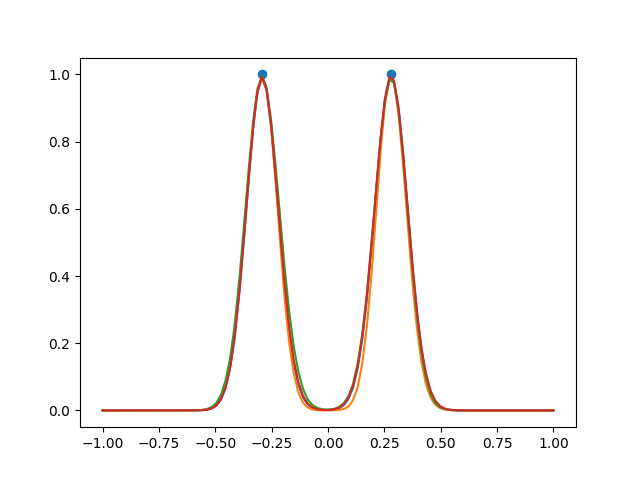
If we do not need the warping function we can obtain the registered curves
directly using the function
landmark_elastic_registration().
If the position of the new location of the landmarks is not specified the mean position is taken.
fd_registered = skfda.preprocessing.registration.landmark_elastic_registration(
    fd,
    landmarks,
)
fd_registered.plot()

plt.scatter(np.mean(landmarks, axis=0), [1, 1])


plt.show()
Ramsay, J., Silverman, B. W. (2005). Functional Data Analysis. Springer.
Ramsay, J., Hooker, G. & Graves S. (2009). Functional Data Analysis with R and Matlab. Springer.
Total running time of the script: (0 minutes 0.229 seconds)