Elastic registration

Shows the usage of the elastic registration to perform a groupwise alignment.

# Author: Pablo Marcos Manchón
# License: MIT

# sphinx_gallery_thumbnail_number = 5

import numpy as np

import skfda
from skfda.datasets import fetch_growth, make_multimodal_samples
from skfda.exploratory.stats import fisher_rao_karcher_mean
from skfda.preprocessing.registration import FisherRaoElasticRegistration

In the example of pairwise alignment was shown the usage of FisherRaoElasticRegistration to align a set of functional observations to a given template or a set of templates.

In the groupwise alignment all the samples are aligned to the same template, constructed to minimise some distance, generally a mean or a median. In the case of the elastic registration, due to the use of the elastic distance in the alignment, one of the most suitable templates is the karcher mean under this metric.

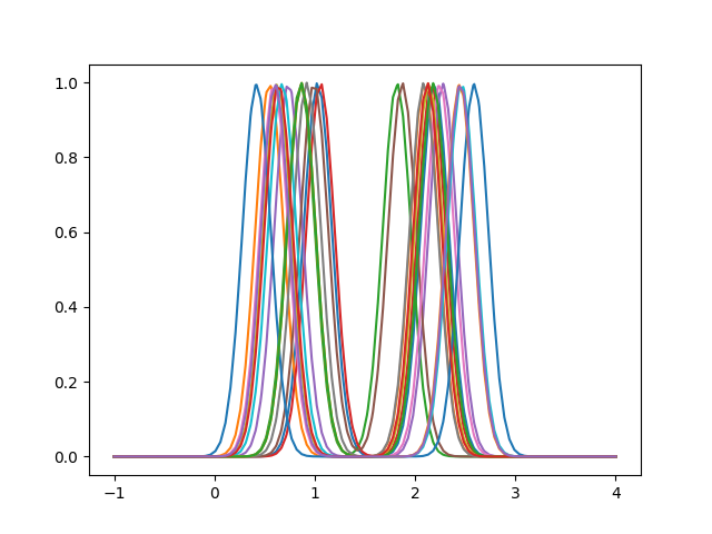
We will create a synthetic dataset to show the basic usage of the registration.

fd = make_multimodal_samples(n_modes=2, stop=4, random_state=1)
fd.plot()

<Figure size 640x480 with 1 Axes>

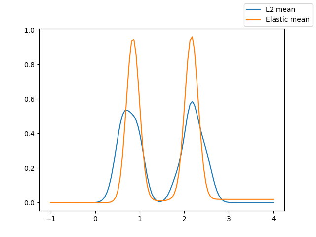
The following figure shows the fisher_rao_karcher_mean() of the dataset and the cross-sectional mean, which correspond to the karcher-mean under the \(\mathbb{L}^2\) distance.

It can be seen how the elastic mean better captures the geometry of the curves compared to the standard mean, since it is not affected by the deformations of the curves.

fig = fd.mean().plot(label="L2 mean")
fisher_rao_karcher_mean(fd).plot(fig=fig, label="Elastic mean")
fig.legend()

<matplotlib.legend.Legend object at 0x7f52b3a8bfd0>

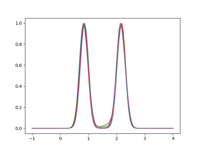
In this case, the alignment completely reduces the amplitude variability between the samples, aligning the maximum points correctly.

elastic_registration = FisherRaoElasticRegistration()

fd_align = elastic_registration.fit_transform(fd)

fd_align.plot()

<Figure size 640x480 with 1 Axes>

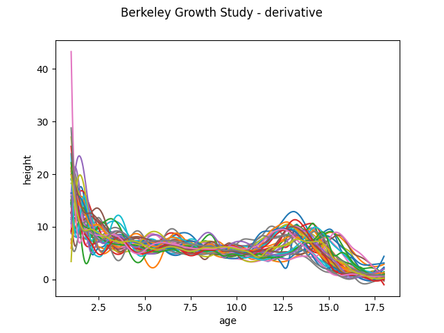
In general these type of alignments are not possible, in the following figure it is shown how it works with a real dataset. The berkeley growth dataset contains the growth curves of a set children, in this case will be used only the males. The growth curves will be resampled using cubic interpolation and derived to obtain the velocity curves.

First we show the original curves:

growth = fetch_growth()

# Select only one sex
fd = growth['data'][growth['target'] == 0]

# Obtain velocity curves
fd.interpolation = skfda.representation.interpolation.SplineInterpolation(3)
fd_derivative = fd.to_grid(np.linspace(*fd.domain_range[0], 200)).derivative()
fd_derivative = fd_derivative.to_grid(np.linspace(*fd.domain_range[0], 50))
fd_derivative.dataset_name = f"{fd.dataset_name} - derivative"
fd_derivative.plot()

<Figure size 640x480 with 1 Axes>

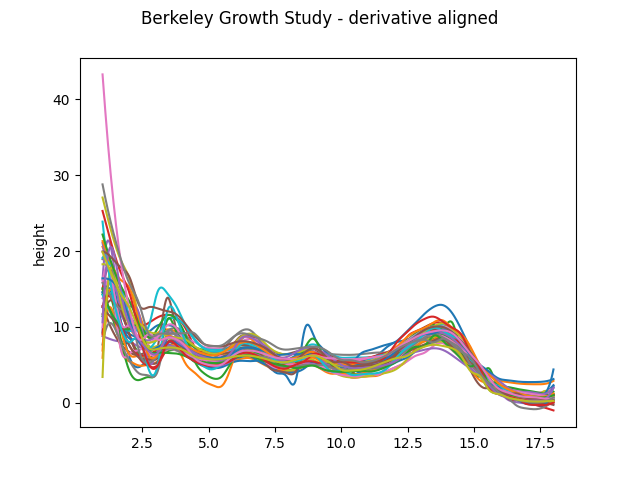
We now show the aligned curves:

fd_align = elastic_registration.fit_transform(fd_derivative)
fd_align.dataset_name = f"{fd.dataset_name} - derivative aligned"

fd_align.plot()

<Figure size 640x480 with 1 Axes>

• Srivastava, Anuj & Klassen, Eric P. (2016). Functional and shape data analysis. In Functional Data and Elastic Registration (pp. 73-122). Springer.

• Tucker, J. D., Wu, W. and Srivastava, A. (2013). Generative Models for Functional Data using Phase and Amplitude Separation. Computational Statistics and Data Analysis, Vol. 61, 50-66.

• J. S. Marron, James O. Ramsay, Laura M. Sangalli and Anuj Srivastava (2015). Functional Data Analysis of Amplitude and Phase Variation. Statistical Science 2015, Vol. 30, No. 4