Extrapolation

Shows the usage of the different types of extrapolation.

# Author: Pablo Marcos Manchón
# License: MIT

# sphinx_gallery_thumbnail_number = 2

import matplotlib.pyplot as plt
import numpy as np

import skfda

The extrapolation defines how to evaluate points that are outside the domain range of a FDataBasis or a FDataGrid.

The FDataBasis objects have a predefined extrapolation which is applied in evaluate if the argument extrapolation is not supplied. This default value could be specified when the object is created or changing the attribute extrapolation.

The extrapolation could be specified by a string with the short name of an extrapolator or with an :class:´~skfda.representation.extrapolation.Extrapolator´.

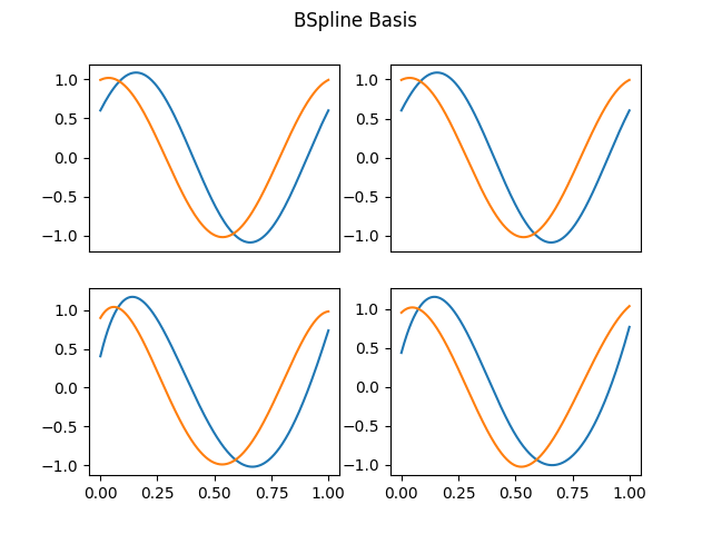
To show how it works we will create a dataset with two unidimensional curves defined in (0,1), and we will represent it using a grid and different types of basis.

fdgrid = skfda.datasets.make_sinusoidal_process(
    n_samples=2,
    error_std=0,
    random_state=0,
)
fdgrid.dataset_name = "Grid"

fd_fourier = fdgrid.to_basis(skfda.representation.basis.FourierBasis())
fd_fourier.dataset_name = "Fourier Basis"

fd_monomial = fdgrid.to_basis(
    skfda.representation.basis.MonomialBasis(n_basis=5),
)
fd_monomial.dataset_name = "Monomial Basis"

fd_bspline = fdgrid.to_basis(
    skfda.representation.basis.BSplineBasis(n_basis=5),
)
fd_bspline.dataset_name = "BSpline Basis"


# Plot of diferent representations
fig, ax = plt.subplots(2, 2)
fdgrid.plot(ax[0][0])
fd_fourier.plot(ax[0][1])
fd_monomial.plot(ax[1][0])
fd_bspline.plot(ax[1][1])

# Disable xticks of first row
ax[0][0].set_xticks([])
ax[0][1].set_xticks([])

# Clear title for next plots
fdgrid.dataset_name = ""

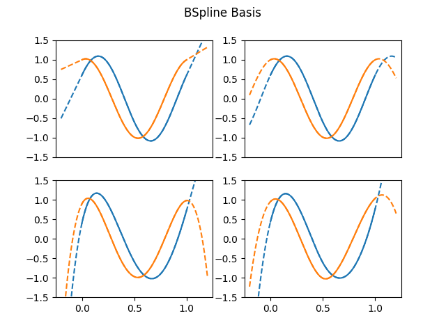
If the extrapolation is not specified when a list of points is evaluated and the default extrapolation of the objects has not been specified it is used the type “none”, which will evaluate the points outside the domain without any kind of control.

For this reason the behavior outside the domain will change depending on the representation, obtaining a periodic behavior in the case of the Fourier basis and polynomial behaviors in the rest of the cases.

domain_extended = (-0.2, 1.2)

fig, ax = plt.subplots(2, 2)


# Plot objects in the domain range extended
fdgrid.plot(ax[0][0], domain_range=domain_extended, linestyle="--")
fd_fourier.plot(ax[0][1], domain_range=domain_extended, linestyle="--")
fd_monomial.plot(ax[1][0], domain_range=domain_extended, linestyle="--")
fd_bspline.plot(ax[1][1], domain_range=domain_extended, linestyle="--")

# Plot configuration
for axes in fig.axes:
    axes.set_prop_cycle(None)
    axes.set_ylim((-1.5, 1.5))
    axes.set_xlim((-0.25, 1.25))

# Disable xticks of first row
ax[0][0].set_xticks([])
ax[0][1].set_xticks([])

# Plot objects in the domain range
fdgrid.plot(ax[0][0])
fd_fourier.plot(ax[0][1])
fd_monomial.plot(ax[1][0])
fd_bspline.plot(ax[1][1])

<Figure size 640x480 with 4 Axes>

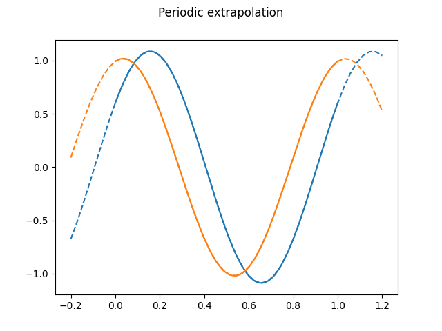
Periodic extrapolation will extend the domain range periodically. The following example shows the periodical extension of an FDataGrid.

It should be noted that the Fourier basis is periodic in itself, but the period does not have to coincide with the domain range, obtaining different results applying or not extrapolation in case of not coinciding.

t = np.linspace(*domain_extended)

fig = plt.figure()
fdgrid.dataset_name = "Periodic extrapolation"

# Evaluation of the grid
# Extrapolation supplied in the evaluation
values = fdgrid(t, extrapolation="periodic")[..., 0]

plt.plot(t, values.T, linestyle="--")

plt.gca().set_prop_cycle(None)  # Reset color cycle

fdgrid.plot(fig=fig)  # Plot dataset

<Figure size 640x480 with 1 Axes>

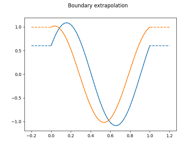
Another possible extrapolation, "bounds", will use the values of the interval bounds for points outside the domain range.

fig = plt.figure()
fdgrid.dataset_name = "Boundary extrapolation"

# Other way to call the extrapolation, changing the default value
fdgrid.extrapolation = "bounds"

# Evaluation of the grid
values = fdgrid(t)[..., 0]
plt.plot(t, values.T, linestyle="--")

plt.gca().set_prop_cycle(None)  # Reset color cycle

fdgrid.plot(fig=fig)  # Plot dataset

<Figure size 640x480 with 1 Axes>

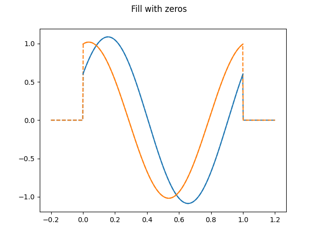
The FillExtrapolation will fill the points extrapolated with the same value. The case of filling with zeros could be specified with the string "zeros", which is equivalent to extrapolation=FillExtrapolation(0).

fdgrid.dataset_name = "Fill with zeros"

# Evaluation of the grid filling with zeros
fdgrid.extrapolation = "zeros"

# Plot in domain extended
fig = fdgrid.plot(domain_range=domain_extended, linestyle="--")

plt.gca().set_prop_cycle(None)  # Reset color cycle

fdgrid.plot(fig=fig)  # Plot dataset

<Figure size 640x480 with 1 Axes>

The string "nan" is equivalent to FillExtrapolation(np.nan).

values = fdgrid([-1, 0, 0.5, 1, 2], extrapolation="nan")
print(values)

[[[        nan]
  [ 0.60293807]
  [-0.60263451]
  [ 0.60293807]
  [        nan]]

 [[        nan]
  [ 0.99401003]
  [-0.99350959]
  [ 0.99401003]
  [        nan]]]

It is possible to configure the extrapolation to raise an exception in case of evaluating a point outside the domain.

try:
    res = fd_fourier(t, extrapolation="exception")
except ValueError as e:
    print(e)

Attempt to evaluate points outside the domain range.

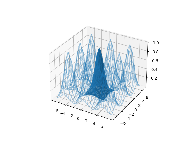
All the extrapolators shown will work with multidimensional objects. In the following example it is constructed a 2d-surface and it is extended using periodic extrapolation.

fig = plt.figure()
ax = fig.add_subplot(111, projection="3d")

# Make data.
t = np.arange(-2.5, 2.75, 0.25)
X, Y = np.meshgrid(t, t)
Z = np.exp(-0.5 * (X**2 + Y**2))

# Creation of FDataGrid
fd_surface = skfda.FDataGrid([Z], (t, t))

t = np.arange(-7, 7.5, 0.5)

# Evaluation with periodic extrapolation
values = fd_surface((t, t), grid=True, extrapolation="periodic")
T, S = np.meshgrid(t, t)


ax.plot_wireframe(T, S, values[0, ..., 0], alpha=0.3, color="C0")
ax.plot_surface(X, Y, Z, color="C0")

<mpl_toolkits.mplot3d.art3d.Poly3DCollection object at 0x7f52b31f7fd0>

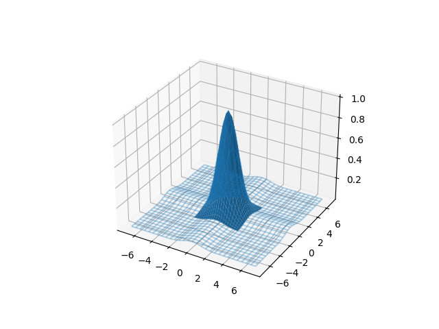
The previous extension can be compared with the extrapolation using the values of the bounds.

values = fd_surface((t, t), grid=True, extrapolation="bounds")

fig = plt.figure()
ax = fig.add_subplot(111, projection="3d")
ax.plot_wireframe(T, S, values[0, ..., 0], alpha=0.3, color="C0")
ax.plot_surface(X, Y, Z, color="C0")

<mpl_toolkits.mplot3d.art3d.Poly3DCollection object at 0x7f52b30220d0>

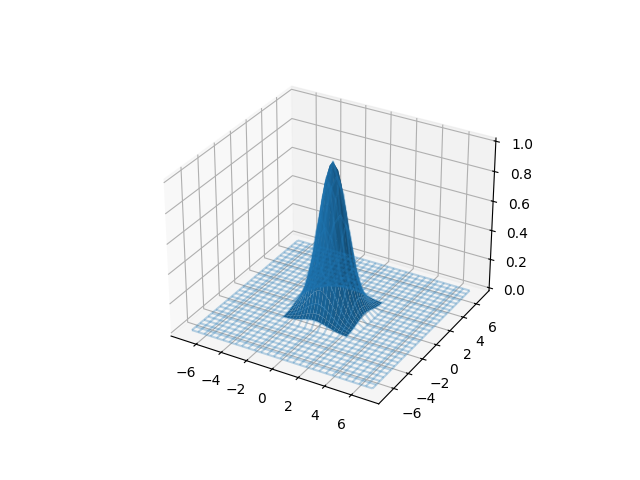
Or filling the surface with zeros outside the domain.

values = fd_surface((t, t), grid=True, extrapolation="zeros")

fig = plt.figure()
ax = fig.add_subplot(111, projection="3d")
ax.plot_wireframe(T, S, values[0, ..., 0], alpha=0.3, color="C0")
ax.plot_surface(X, Y, Z, color="C0")

<mpl_toolkits.mplot3d.art3d.Poly3DCollection object at 0x7f52966dba00>