One-way functional ANOVA with synthetic data

This example shows how to perform a functional one-way ANOVA test with synthetic data.

# Author: David García Fernández
# License: MIT


from skfda.datasets import make_gaussian_process
from skfda.inference.anova import oneway_anova
from skfda.misc.covariances import WhiteNoise
from skfda.representation import FDataGrid

import numpy as np

One-way ANOVA (analysis of variance) is a test that can be used to compare the means of different samples of data. Let \(X_{ij}(t), j=1, \dots, n_i\) be trajectories corresponding to \(k\) independent samples \((i=1,\dots,k)\) and let \(E(X_i(t)) = m_i(t)\). Thus, the null hypothesis in the statistical test is:

\[H_0: m_1(t) = \dots = m_k(t)\]

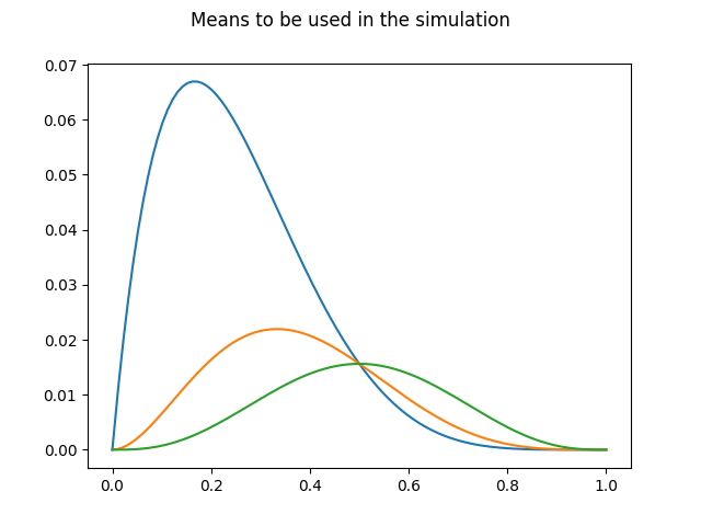
In this example we will explain the nature of ANOVA method and its behavior under certain conditions simulating data. Specifically, we will generate three different trajectories, for each one we will simulate a stochastic process by adding to them white noise. The main objective of the test is to illustrate the differences in the results of the ANOVA method when the covariance function of the brownian processes changes.

First, the means for the future processes are drawn.

n_samples = 10
n_features = 100
n_groups = 3
start = 0
stop = 1

t = np.linspace(start, stop, n_features)

m1 = t * (1 - t) ** 5
m2 = t ** 2 * (1 - t) ** 4
m3 = t ** 3 * (1 - t) ** 3

_ = FDataGrid([m1, m2, m3],
              dataset_name="Means to be used in the simulation").plot()

A total of n_samples trajectories will be created for each mean, so an array of labels is created to identify them when plotting.

groups = np.full(n_samples * n_groups, 'Sample 1')
groups[10:20] = 'Sample 2'
groups[20:] = 'Sample 3'

First simulation uses a low \(\sigma^2 = 0.01\) value. In this case the differences between the means of each group should be clear, and the p-value for the test should be near to zero.

sigma2 = 0.01
cov = WhiteNoise(variance=sigma2)

fd1 = make_gaussian_process(n_samples, mean=m1, cov=cov,
                            n_features=n_features, random_state=1, start=start,
                            stop=stop)
fd2 = make_gaussian_process(n_samples, mean=m2, cov=cov,
                            n_features=n_features, random_state=2, start=start,
                            stop=stop)
fd3 = make_gaussian_process(n_samples, mean=m3, cov=cov,
                            n_features=n_features, random_state=3, start=start,
                            stop=stop)
stat, p_val = oneway_anova(fd1, fd2, fd3, random_state=4)
print("Statistic: {:.3f}".format(stat))
print("p-value: {:.3f}".format(p_val))

Statistic: 0.082
p-value: 0.074

In the following, the same process will be followed incrementing sigma value, this way the differences between the averages of each group will be lower and the p-values will increase (the null hypothesis will be harder to refuse).

Plot for \(\sigma^2 = 0.1\):

sigma2 = 0.1
cov = WhiteNoise(variance=sigma2)

fd1 = make_gaussian_process(n_samples, mean=m1, cov=cov,
                            n_features=n_features, random_state=1, start=t[0],
                            stop=t[-1])
fd2 = make_gaussian_process(n_samples, mean=m2, cov=cov,
                            n_features=n_features, random_state=2, start=t[0],
                            stop=t[-1])
fd3 = make_gaussian_process(n_samples, mean=m3, cov=cov,
                            n_features=n_features, random_state=3, start=t[0],
                            stop=t[-1])

stat, p_val = oneway_anova(fd1, fd2, fd3, random_state=4)
print("Statistic: {:.3f}".format(stat))
print("p-value: {:.3f}".format(p_val))

Statistic: 0.653
p-value: 0.329

Plot for \(\sigma^2 = 1\):

sigma2 = 1
cov = WhiteNoise(variance=sigma2)

fd1 = make_gaussian_process(n_samples, mean=m1, cov=cov,
                            n_features=n_features, random_state=1, start=t[0],
                            stop=t[-1])
fd2 = make_gaussian_process(n_samples, mean=m2, cov=cov,
                            n_features=n_features, random_state=2, start=t[0],
                            stop=t[-1])
fd3 = make_gaussian_process(n_samples, mean=m3, cov=cov,
                            n_features=n_features, random_state=3, start=t[0],
                            stop=t[-1])

stat, p_val = oneway_anova(fd1, fd2, fd3, random_state=4)
print("Statistic: {:.3f}".format(stat))
print("p-value: {:.3f}".format(p_val))

Statistic: 6.304
p-value: 0.395

References:

[1] Antonio Cuevas, Manuel Febrero-Bande, and Ricardo Fraiman. “An anova test for functional data”. Computational Statistics Data Analysis, 47:111-112, 02 2004