Kernel Regression

In this example we will see and compare the performance of different kernel regression methods.

# Author: Elena Petrunina
# License: MIT

import numpy as np
from sklearn.metrics import r2_score
from sklearn.model_selection import GridSearchCV, train_test_split

import skfda
from skfda.misc.hat_matrix import (
    KNeighborsHatMatrix,
    LocalLinearRegressionHatMatrix,
    NadarayaWatsonHatMatrix,
)
from skfda.ml.regression._kernel_regression import KernelRegression

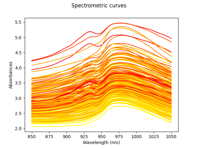
For this example, we will use the tecator dataset. This data set contains 215 samples. For each sample the data consists of a spectrum of absorbances and the contents of water, fat and protein.

X, y = skfda.datasets.fetch_tecator(return_X_y=True, as_frame=True)
X = X.iloc[:, 0].values
fat = y['fat'].values

Fat percentages will be estimated from the spectrum. All curves are shown in the image above. The color of these depends on the amount of fat, from least (yellow) to highest (red).

X.plot(gradient_criteria=fat, legend=True)

<Figure size 640x480 with 1 Axes>

The data set is splitted into train and test sets with 80% and 20% of the samples respectively.

X_train, X_test, y_train, y_test = train_test_split(
    X,
    fat,
    test_size=0.2,
    random_state=1,
)

The KNN hat matrix will be tried first. We will use the default kernel function, i.e. uniform kernel. To find the most suitable number of neighbours GridSearchCV will be used, testing with any number from 1 to 100.

n_neighbors = np.array(range(1, 100))
knn = GridSearchCV(
    KernelRegression(kernel_estimator=KNeighborsHatMatrix()),
    param_grid={'kernel_estimator__n_neighbors': n_neighbors},
)

The best performance for the train set is obtained with the following number of neighbours

knn.fit(X_train, y_train)
print(
    'KNN bandwidth:',
    knn.best_params_['kernel_estimator__n_neighbors'],
)

KNN bandwidth: 3

The accuracy of the estimation using r2_score measurement on the test set is shown below.

y_pred = knn.predict(X_test)
knn_res = r2_score(y_pred, y_test)
print('Score KNN:', knn_res)

Score KNN: 0.3500795818805428

Following a similar procedure for Nadaraya-Watson, the optimal parameter is chosen from the interval (0.01, 1).

bandwidth = np.logspace(-2, 0, num=100)
nw = GridSearchCV(
    KernelRegression(kernel_estimator=NadarayaWatsonHatMatrix()),
    param_grid={'kernel_estimator__bandwidth': bandwidth},
)

The best performance is obtained with the following bandwidth

nw.fit(X_train, y_train)
print(
    'Nadaraya-Watson bandwidth:',
    nw.best_params_['kernel_estimator__bandwidth'],
)

Nadaraya-Watson bandwidth: 0.37649358067924693

The accuracy of the estimation is shown below and should be similar to that obtained with the KNN method.

y_pred = nw.predict(X_test)
nw_res = r2_score(y_pred, y_test)
print('Score NW:', nw_res)

Score NW: 0.3127155617541537

For Local Linear Regression, FDataBasis representation with a basis should be used (for the previous cases it is possible to use either FDataGrid or FDataBasis).

For basis, Fourier basis with 10 elements has been selected. Note that the number of functions in the basis affects the estimation result and should ideally also be chosen using cross-validation.

fourier = skfda.representation.basis.FourierBasis(n_basis=10)

X_basis = X.to_basis(basis=fourier)
X_basis_train, X_basis_test, y_train, y_test = train_test_split(
    X_basis,
    fat,
    test_size=0.2,
    random_state=1,
)


bandwidth = np.logspace(0.3, 1, num=100)

llr = GridSearchCV(
    KernelRegression(kernel_estimator=LocalLinearRegressionHatMatrix()),
    param_grid={'kernel_estimator__bandwidth': bandwidth},
)

The bandwidth obtained by cross-validation is indicated below.

llr.fit(X_basis_train, y_train)
print(
    'LLR bandwidth:',
    llr.best_params_['kernel_estimator__bandwidth'],
)

LLR bandwidth: 4.7287621998304505

Although it is a slower method, the result obtained in this example should be better than in the case of Nadaraya-Watson and KNN.

y_pred = llr.predict(X_basis_test)
llr_res = r2_score(y_pred, y_test)
print('Score LLR:', llr_res)

Score LLR: 0.9731955244187162

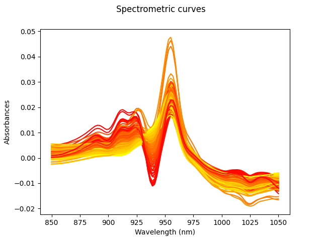
For this data set using the derivative should give a better performance.

Below the plot of all the derivatives can be found. The same scheme as before is followed: yellow les fat, red more.

Xd = X.derivative()
Xd.plot(gradient_criteria=fat, legend=True)

Xd_train, Xd_test, y_train, y_test = train_test_split(
    Xd,
    fat,
    test_size=0.2,
    random_state=1,
)

Exactly the same operations are repeated, but now with the derivatives of the functions.

K-Nearest Neighbours

knn = GridSearchCV(
    KernelRegression(kernel_estimator=KNeighborsHatMatrix()),
    param_grid={'kernel_estimator__n_neighbors': n_neighbors},
)

knn.fit(Xd_train, y_train)
print(
    'KNN bandwidth:',
    knn.best_params_['kernel_estimator__n_neighbors'],
)

y_pred = knn.predict(Xd_test)
dknn_res = r2_score(y_pred, y_test)
print('Score KNN:', dknn_res)

KNN bandwidth: 4
Score KNN: 0.9428247359478524

Nadaraya-Watson

bandwidth = np.logspace(-3, -1, num=100)
nw = GridSearchCV(
    KernelRegression(kernel_estimator=NadarayaWatsonHatMatrix()),
    param_grid={'kernel_estimator__bandwidth': bandwidth},
)

nw.fit(Xd_train, y_train)
print(
    'Nadara-Watson bandwidth:',
    nw.best_params_['kernel_estimator__bandwidth'],
)

y_pred = nw.predict(Xd_test)
dnw_res = r2_score(y_pred, y_test)
print('Score NW:', dnw_res)

Nadara-Watson bandwidth: 0.006135907273413175
Score NW: 0.9491787548158307

For both Nadaraya-Watson and KNN the accuracy has improved significantly and should be higher than 0.9.

Local Linear Regression

Xd_basis = Xd.to_basis(basis=fourier)
Xd_basis_train, Xd_basis_test, y_train, y_test = train_test_split(
    Xd_basis,
    fat,
    test_size=0.2,
    random_state=1,
)

bandwidth = np.logspace(-2, 1, 100)
llr = GridSearchCV(
    KernelRegression(kernel_estimator=LocalLinearRegressionHatMatrix()),
    param_grid={'kernel_estimator__bandwidth': bandwidth},
)

llr.fit(Xd_basis_train, y_train)
print(
    'LLR bandwidth:',
    llr.best_params_['kernel_estimator__bandwidth'],
)

y_pred = llr.predict(Xd_basis_test)
dllr_res = r2_score(y_pred, y_test)
print('Score LLR:', dllr_res)

LLR bandwidth: 0.010722672220103232
Score LLR: 0.9949460304758446

LLR accuracy has also improved, but the difference with Nadaraya-Watson and KNN in the case of derivatives is less significant than in the previous case.