Kernel Smoothing

This example uses different kernel smoothing methods over the phoneme data set (phoneme) and shows how cross validations scores vary over a range of different parameters used in the smoothing methods. It also shows examples of undersmoothing and oversmoothing.

# Author: Miguel Carbajo Berrocal
# Modified: Elena Petrunina
# License: MIT
import math

import matplotlib.pyplot as plt
import numpy as np

import skfda
from skfda.misc.hat_matrix import (
    KNeighborsHatMatrix,
    LocalLinearRegressionHatMatrix,
    NadarayaWatsonHatMatrix,
)
from skfda.misc.kernels import uniform
from skfda.preprocessing.smoothing import KernelSmoother
from skfda.preprocessing.smoothing.validation import SmoothingParameterSearch

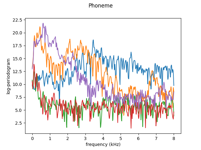
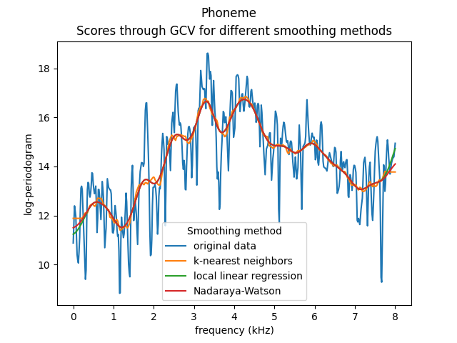
This dataset contains the log-periodograms of several phoneme pronunciations. The phoneme curves are very irregular and noisy, so we usually will want to smooth them as a preprocessing step.

As an example, we will smooth the first 300 curves only. In the following plot, the first five curves are shown.

dataset = skfda.datasets.fetch_phoneme()
fd = dataset['data'][:300]

fd[:5].plot()
plt.show()

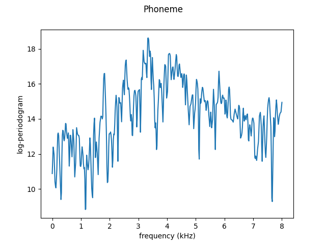
To better illustrate the smoothing effects and the influence of different values of the bandwidth parameter, all results will be plotted for a single curve. However, note that the smoothing is performed at the same time for all functions contained in a FData object.

We will take the curve found at index 10 (a random choice). Below the original (without any smoothing) curve is plotted.

fd[10].plot()
plt.show()

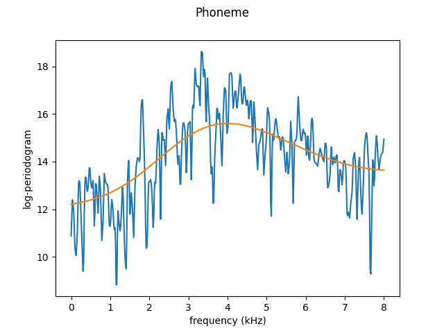
The library currently has three smoothing methods available: Nadaraya-Watson, Local Linear Regression and K-Neigbors.

The bandwith parameter controls the influence of more distant points on the final estimation. So, it is to be expected that with larger bandwidth values, the resulting function will be smoother.

Below are examples of oversmoothing (with bandwidth = 1) and undersmoothing (with bandwidth = 0.05) using the Nadaraya-Watson method with normal kernel.

fd_os = KernelSmoother(
    kernel_estimator=NadarayaWatsonHatMatrix(bandwidth=1),
).fit_transform(fd)

fd_us = KernelSmoother(
    kernel_estimator=NadarayaWatsonHatMatrix(bandwidth=0.05),
).fit_transform(fd)

Over-smoothed

fig = fd[10].plot()
fd_os[10].plot(fig=fig)
plt.show()

Under-smoothed

fig = fd[10].plot()
fd_us[10].plot(fig=fig)
plt.show()

The same could be done with different kernel. For example, over-smoothed case with uniform kernel:

fd_os = KernelSmoother(
    kernel_estimator=NadarayaWatsonHatMatrix(bandwidth=1, kernel=uniform),
).fit_transform(fd)

fig = fd[10].plot()
fd_os[10].plot(fig=fig)
plt.show()

The values for which the undersmoothing and oversmoothing occur are different for each dataset and that is why the library also has parameter search methods.

Here we show the general cross validation scores for different values of the parameters given to the different smoothing methods.

The smoothing parameter for k-NN is the number of neighbors. We will choose this parameter between 2 and 23 in this example.

n_neighbors = np.arange(2, 24)

The smoothing parameter for Nadaraya Watson and Local Linear Regression is a bandwidth parameter, with the same units as the domain of the function. As we want to compare the results of these smoothers with k-NN, with uses as the smoothing parameter the number of neighbors, we want to use a comparable range of values. In this case, we know that our grid points are equispaced and the distance between two contiguous points is approximately 0.03.

As we want to obtain the estimate at the same points where the function is already defined (input_points equals output_points), the nearest neighbor will be the point itself, and the second nearest neighbor, the contiguous point. So to get equivalent bandwidth values for each value of n_neigbors we have to take 22 values in the range from approximately 0.3 to 0.3*11

dist = fd.grid_points[0][1] - fd.grid_points[0][0]
bandwidth = np.linspace(
    dist,
    dist * (math.ceil((n_neighbors[-1] - 1) / 2)),
    len(n_neighbors),
)

# K-nearest neighbours kernel smoothing.

knn = SmoothingParameterSearch(
    KernelSmoother(kernel_estimator=KNeighborsHatMatrix()),
    n_neighbors,
    param_name='kernel_estimator__n_neighbors',
)
knn.fit(fd)
knn_fd = knn.transform(fd)

# Local linear regression kernel smoothing.
llr = SmoothingParameterSearch(
    KernelSmoother(kernel_estimator=LocalLinearRegressionHatMatrix()),
    bandwidth,
    param_name='kernel_estimator__bandwidth',
)
llr.fit(fd)
llr_fd = llr.transform(fd)

# Nadaraya-Watson kernel smoothing.
nw = SmoothingParameterSearch(
    KernelSmoother(kernel_estimator=NadarayaWatsonHatMatrix()),
    bandwidth,
    param_name='kernel_estimator__bandwidth',
)
nw.fit(fd)
nw_fd = nw.transform(fd)

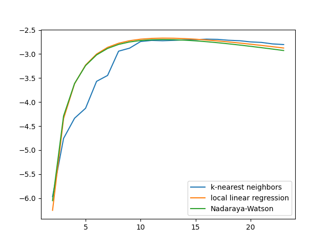
For more information on how the parameter search is performed and how score is calculated see LinearSmootherGeneralizedCVScorer

The plot of the mean test scores for all smoothers is shown below. As the X axis we will use the neighbors for all the smoothers in order to compare k-NN with the others, but remember that the bandwidth for the other two estimators, in this case, is related to the distance to the k-th neighbor.

fig = plt.figure()
ax = fig.add_subplot(1, 1, 1)
ax.plot(
    n_neighbors,
    knn.cv_results_['mean_test_score'],
    label='k-nearest neighbors',
)
ax.plot(
    n_neighbors,
    llr.cv_results_['mean_test_score'],
    label='local linear regression',
)
ax.plot(
    n_neighbors,
    nw.cv_results_['mean_test_score'],
    label='Nadaraya-Watson',
)
ax.legend()
plt.show()

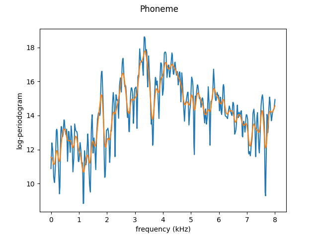
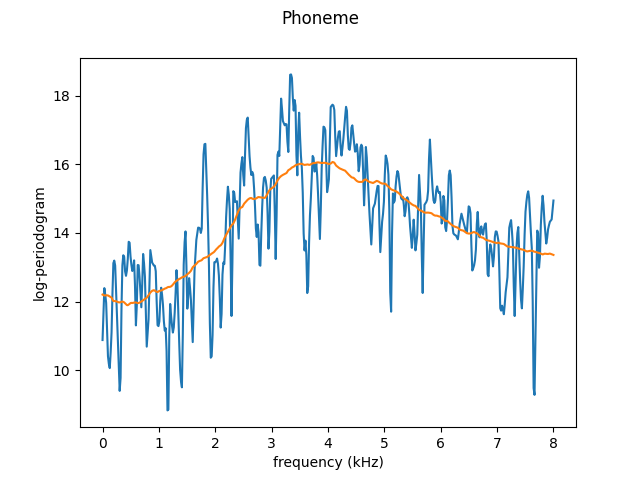
We can plot the smoothed curves corresponding to the 11th element of the data set for the three different smoothing methods.

fig = plt.figure()
ax = fig.add_subplot(1, 1, 1)
ax.set_xlabel('Smoothing method parameter')
ax.set_ylabel('GCV score')
ax.set_title('Scores through GCV for different smoothing methods')

fd[10].plot(fig=fig)
knn_fd[10].plot(fig=fig)
llr_fd[10].plot(fig=fig)
nw_fd[10].plot(fig=fig)
ax.legend(
    [
        'original data',
        'k-nearest neighbors',
        'local linear regression',
        'Nadaraya-Watson',
    ],
    title='Smoothing method',
)
plt.show()

Now, we can see the effects of a proper smoothing. We can plot the same 5 samples from the beginning using the Nadaraya-Watson kernel smoother with the best choice of parameter.

fig, ax = plt.subplots(2)
fd[:5].plot(ax[0])
nw_fd[:5].plot(ax[1])
# Disable xticks and xlabel of first image
ax[0].set_xticks([])
ax[0].set_xlabel('')
plt.show()