Neighbors Scalar Regression

Shows the usage of the nearest neighbors regressor with scalar response.

# Author: Pablo Marcos Manchón
# License: MIT

# sphinx_gallery_thumbnail_number = 3

import matplotlib.pyplot as plt
import numpy as np
from sklearn.model_selection import GridSearchCV, train_test_split

import skfda
from skfda.ml.regression import KNeighborsRegressor

In this example, we are going to show the usage of the nearest neighbors regressors with scalar response. There is available a K-nn version, KNeighborsRegressor, and other one based in the radius, RadiusNeighborsRegressor.

Firstly we will fetch a dataset to show the basic usage.

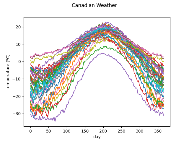
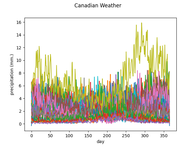
The Canadian weather dataset contains the daily temperature and precipitation at 35 different locations in Canada averaged over 1960 to 1994.

The following figure shows the different temperature and precipitation curves.

data = skfda.datasets.fetch_weather()
fd = data['data']


# Split dataset, temperatures and curves of precipitation
X, y_func = fd.coordinates

Temperatures

X.plot()

<Figure size 640x480 with 1 Axes>

Precipitation

y_func.plot()

<Figure size 640x480 with 1 Axes>

We will try to predict the total log precipitation, i.e, \(logPrecTot_i = \log \sum_{t=0}^{365} prec_i(t)\) using the temperature curves.

# Sum directly from the data matrix
prec = y_func.data_matrix.sum(axis=1)[:, 0]
log_prec = np.log(prec)

print(log_prec)

[7.30033776 7.28276118 7.29600641 7.14084916 7.0914925  7.02811278
 6.6861106  6.79860983 6.83668883 7.09721794 7.01148446 6.84673058
 6.81640724 6.66262171 6.86484778 6.5572044  6.23284087 6.10724558
 6.01322604 5.91647157 6.0078299  5.89357605 6.14246742 5.99271377
 5.60543435 7.0519422  6.74711693 6.41165405 7.86010789 5.60469852
 5.79209856 5.59136005 6.02707297 5.56106617 4.9698133 ]

As in the nearest neighbors classifier examples, we will split the dataset in two partitions, for training and test, using the sklearn function train_test_split().

X_train, X_test, y_train, y_test = train_test_split(
    X,
    log_prec,
    random_state=7,
)

Firstly we will try make a prediction with the default values of the estimator, using 5 neighbors and the \(\mathbb{L}^2\) distance.

We can fit the KNeighborsRegressor in the same way than the sklearn estimators. This estimator is an extension of the sklearn KNeighborsRegressor, but accepting a FDataGrid as input instead of an array with multivariate data.

knn = KNeighborsRegressor(weights='distance')
knn.fit(X_train, y_train)

KNeighborsRegressor(weights='distance')

In a Jupyter environment, please rerun this cell to show the HTML representation or trust the notebook.
On GitHub, the HTML representation is unable to render, please try loading this page with nbviewer.org.

We can predict values for the test partition using predict().

pred = knn.predict(X_test)
print(pred)

[7.11225785 5.99768933 7.05559273 6.88718564 6.78535172 5.97132028
 6.56125279 6.47991884 6.92965595]

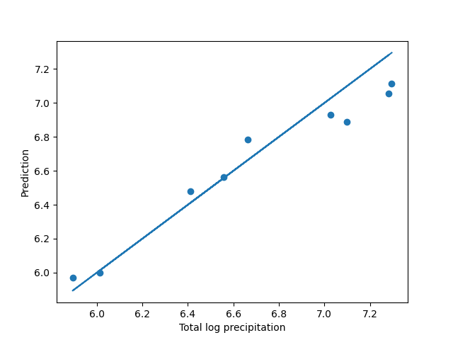
The following figure compares the real precipitations with the predicted values.

fig = plt.figure()
ax = fig.add_subplot(1, 1, 1)
ax.scatter(y_test, pred)
ax.plot(y_test, y_test)
ax.set_xlabel("Total log precipitation")
ax.set_ylabel("Prediction")

Text(42.597222222222214, 0.5, 'Prediction')

We can quantify how much variability it is explained by the model with the coefficient of determination \(R^2\) of the prediction, using score() for that.

The coefficient \(R^2\) is defined as \((1 - u/v)\), where \(u\) is the residual sum of squares \(\sum_i (y_i - y_{pred_i})^ 2\) and \(v\) is the total sum of squares \(\sum_i (y_i - \bar y )^2\).

score = knn.score(X_test, y_test)
print(score)

0.9244558571515601

In this case, we obtain a really good aproximation with this naive approach, although, due to the small number of samples, the results will depend on how the partition was done. In the above case, the explained variation is inflated for this reason.

We will perform cross-validation to test more robustly our model.

Also, we can make a grid search, using GridSearchCV, to determine the optimal number of neighbors and the best way to weight their votes.

param_grid = {
    'n_neighbors': range(1, 12, 2),
    'weights': ['uniform', 'distance'],
}


knn = KNeighborsRegressor()
gscv = GridSearchCV(
    knn,
    param_grid,
    cv=5,
)
gscv.fit(X, log_prec)

GridSearchCV(cv=5, estimator=KNeighborsRegressor(),
             param_grid={'n_neighbors': range(1, 12, 2),
                         'weights': ['uniform', 'distance']})

In a Jupyter environment, please rerun this cell to show the HTML representation or trust the notebook.
On GitHub, the HTML representation is unable to render, please try loading this page with nbviewer.org.

We obtain that 7 is the optimal number of neighbors.

print("Best params", gscv.best_params_)
print("Best score", gscv.best_score_)

Best params {'n_neighbors': 3, 'weights': 'distance'}
Best score -2.5211096524610666

More detailed information about the Canadian weather dataset can be obtained in the following references.

• Ramsay, James O., and Silverman, Bernard W. (2006). Functional Data Analysis, 2nd ed. , Springer, New York.

• Ramsay, James O., and Silverman, Bernard W. (2002). Applied Functional Data Analysis, Springer, New Yorkn’