Radius neighbors classification

Shows the usage of the radius nearest neighbors classifier.

# Author: Pablo Marcos Manchón
# License: MIT

# sphinx_gallery_thumbnail_number = 2


import numpy as np
from sklearn.model_selection import train_test_split

import skfda
from skfda.misc.metrics import PairwiseMetric, linf_distance
from skfda.ml.classification import RadiusNeighborsClassifier

In this example, we are going to show the usage of the radius nearest neighbors classifier in their functional version, a variation of the K-nearest neighbors classifier, where it is used a vote among neighbors within a given radius, instead of use the k nearest neighbors.

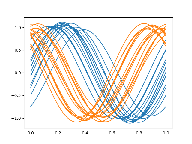
Firstly, we will construct a toy dataset to show the basic usage of the API. We will create two classes of sinusoidal samples, with different phases.

Make toy dataset

fd1 = skfda.datasets.make_sinusoidal_process(
    error_std=0,
    phase_std=0.35,
    random_state=0,
)
fd2 = skfda.datasets.make_sinusoidal_process(
    phase_mean=1.9,
    error_std=0,
    random_state=1,
)

X = fd1.concatenate(fd2)
y = np.array(15 * [0] + 15 * [1])

# Plot toy dataset
X.plot(group=y, group_colors=['C0', 'C1'])

<Figure size 640x480 with 1 Axes>

As in the K-nearest neighbor example, we will split the dataset in two partitions, for training and test, using the sklearn function train_test_split().

# Concatenate the two classes in the same FDataGrid.

X_train, X_test, y_train, y_test = train_test_split(
    X,
    y,
    test_size=0.25,
    shuffle=True,
    stratify=y,
    random_state=0,
)

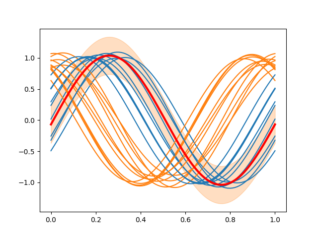
The label assigned to a test sample will be the majority class of its neighbors, in this case all the samples in the ball center in the sample.

If we use the \(\mathbb{L}^\infty\) metric, we can visualize a ball as a bandwidth with a fixed radius around a function. The following figure shows the ball centered in the first sample of the test partition.

radius = 0.3
sample = X_test[0]  # Center of the ball

fig = X_train.plot(group=y_train, group_colors=['C0', 'C1'])

# Plot ball
sample.plot(fig=fig, color='red', linewidth=3)
lower = sample - radius
upper = sample + radius
fig.axes[0].fill_between(
    sample.grid_points[0],
    lower.data_matrix.flatten(),
    upper.data_matrix[0].flatten(),
    alpha=0.25,
    color='C1',
)

<matplotlib.collections.PolyCollection object at 0x7f52965ed790>

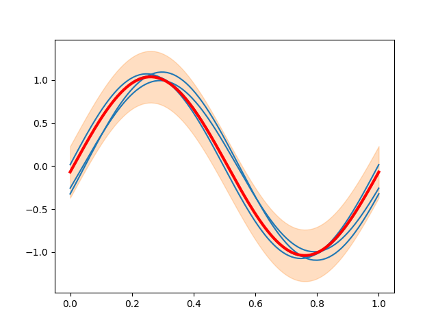
In this case, all the neighbors in the ball belong to the first class, so this will be the class predicted.

# Creation of pairwise distance
l_inf = PairwiseMetric(linf_distance)
distances = l_inf(sample, X_train)[0]  # L_inf distances to 'sample'

# Plot samples in the ball
fig = X_train[distances <= radius].plot(color='C0')
sample.plot(fig=fig, color='red', linewidth=3)
fig.axes[0].fill_between(
    sample.grid_points[0],
    lower.data_matrix.flatten(),
    upper.data_matrix[0].flatten(),
    alpha=0.25,
    color='C1',
)

<matplotlib.collections.PolyCollection object at 0x7f52b3bb7190>

We will fit the classifier RadiusNeighborsClassifier, which has a similar API than the sklearn estimator RadiusNeighborsClassifier but accepting FDataGrid instead of arrays with multivariate data.

The vote of the neighbors can be weighted using the paramenter weights. In this case we will weight the vote inversely proportional to the distance.

radius_nn = RadiusNeighborsClassifier(radius=radius, weights='distance')
radius_nn.fit(X_train, y_train)

RadiusNeighborsClassifier(radius=0.3, weights='distance')

In a Jupyter environment, please rerun this cell to show the HTML representation or trust the notebook.
On GitHub, the HTML representation is unable to render, please try loading this page with nbviewer.org.

We can predict labels for the test partition with predict().

pred = radius_nn.predict(X_test)
print(pred)

[0 0 0 1 1 1 1 0]

In this case, we get 100% accuracy, although it is a toy dataset.

test_score = radius_nn.score(X_test, y_test)
print(test_score)

1.0

If the radius is too small, it is possible to get samples with no neighbors. The classifier will raise and exception in this case.

radius_nn.set_params(radius=0.5)  #  Radius 0.05 in the L2 distance
radius_nn.fit(X_train, y_train)

try:
    radius_nn.predict(X_test)
except ValueError as e:
    print(e)

A label to these oulier samples can be provided to avoid this problem.

radius_nn.set_params(outlier_label=2)
radius_nn.fit(X_train, y_train)
pred = radius_nn.predict(X_test)

print(pred)

[0 0 0 1 1 1 1 0]

This classifier can be used with multivariate funcional data, as surfaces or curves in \(\mathbb{R}^N\), if the metric support it too.