Functional Principal Component Analysis

Explores the two possible ways to do functional principal component analysis.

# Author: Yujian Hong
# License: MIT

import matplotlib.pyplot as plt

import skfda
from skfda.datasets import fetch_growth
from skfda.exploratory.visualization import FPCAPlot
from skfda.preprocessing.dim_reduction import FPCA
from skfda.representation.basis import (
    BSplineBasis,
    FourierBasis,
    MonomialBasis,
)

In this example we are going to use functional principal component analysis to explore datasets and obtain conclusions about said dataset using this technique.

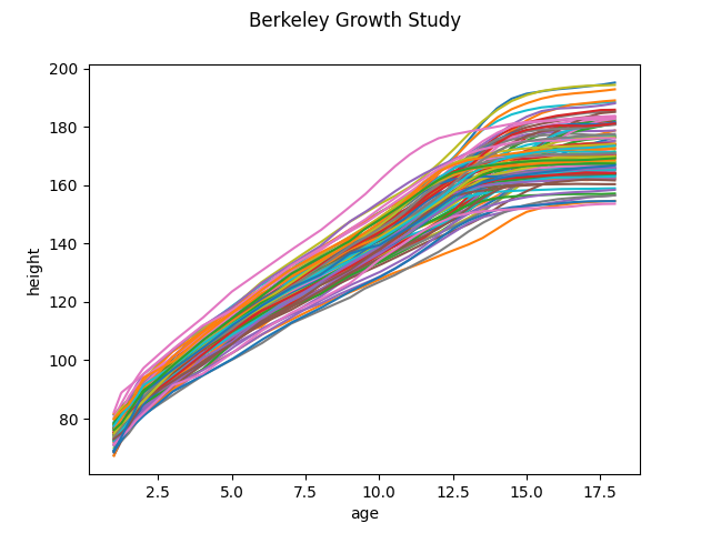
First we are going to fetch the Berkeley Growth Study data. This dataset correspond to the height of several boys and girls measured from birth to when they are 18 years old. The number and time of the measurements are the same for each individual. To better understand the data we plot it.

dataset = skfda.datasets.fetch_growth()
fd = dataset['data']
y = dataset['target']
fd.plot()

<Figure size 640x480 with 1 Axes>

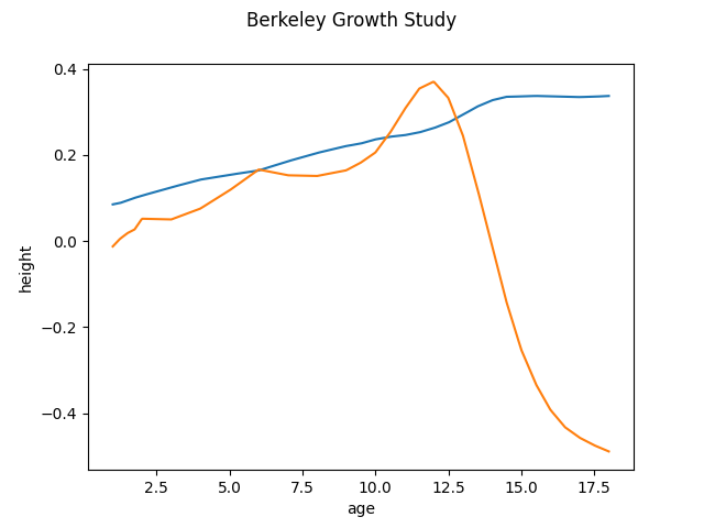
FPCA can be done in two ways. The first way is to operate directly with the raw data. We call it discretized FPCA as the functional data in this case consists in finite values dispersed over points in a domain range. We initialize and setup the FPCADiscretized object and run the fit method to obtain the first two components. By default, if we do not specify the number of components, it’s 3. Other parameters are weights and centering. For more information please visit the documentation.

fpca_discretized = FPCA(n_components=2)
fpca_discretized.fit(fd)
fpca_discretized.components_.plot()

<Figure size 640x480 with 1 Axes>

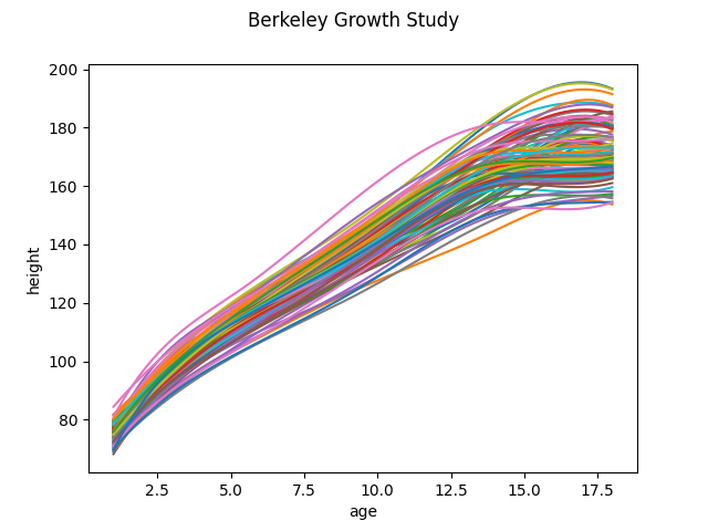
In the second case, the data is first converted to use a basis representation and the FPCA is done with the basis representation of the original data. We obtain the same dataset again and transform the data to a basis representation. This is because the FPCA module modifies the original data. We also plot the data for better visual representation.

dataset = fetch_growth()
fd = dataset['data']
basis = skfda.representation.basis.BSplineBasis(n_basis=7)
basis_fd = fd.to_basis(basis)
basis_fd.plot()

<Figure size 640x480 with 1 Axes>

We initialize the FPCABasis object and run the fit function to obtain the first 2 principal components. By default the principal components are expressed in the same basis as the data. We can see that the obtained result is similar to the discretized case.

fpca = FPCA(n_components=2)
fpca.fit(basis_fd)
fpca.components_.plot()

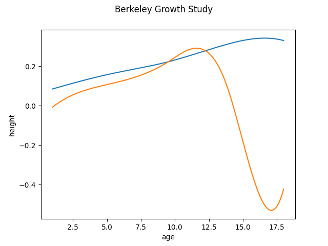
<Figure size 640x480 with 1 Axes>

To better illustrate the effects of the obtained two principal components, we add and subtract a multiple of the components to the mean function. We can then observe now that this principal component represents the variation in the mean growth between the children. The second component is more interesting. The most appropriate explanation is that it represents the differences between girls and boys. Girls tend to grow faster at an early age and boys tend to start puberty later, therefore, their growth is more significant later. Girls also stop growing early

FPCAPlot(
    basis_fd.mean(),
    fpca.components_,
    factor=30,
    fig=plt.figure(figsize=(6, 2 * 4)),
    n_rows=2,
).plot()

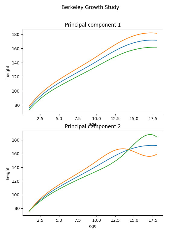
<Figure size 600x800 with 2 Axes>

We can also specify another basis for the principal components as argument when creating the FPCABasis object. For example, if we use the Fourier basis for the obtained principal components we can see that the components are periodic. This example is only to illustrate the effect. In this dataset, as the functions are not periodic it does not make sense to use the Fourier basis

dataset = fetch_growth()
fd = dataset['data']
basis_fd = fd.to_basis(BSplineBasis(n_basis=7))
fpca = FPCA(n_components=2, components_basis=FourierBasis(n_basis=7))
fpca.fit(basis_fd)
fpca.components_.plot()

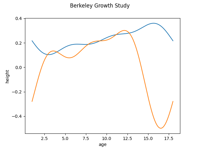
<Figure size 640x480 with 1 Axes>

We can observe that if we switch to the Monomial basis, we also lose the key features of the first principal components because it distorts the principal components, adding extra maximums and minimums. Therefore, in this case the best option is to use the BSpline basis as the basis for the principal components

dataset = fetch_growth()
fd = dataset['data']
basis_fd = fd.to_basis(BSplineBasis(n_basis=7))
fpca = FPCA(n_components=2, components_basis=MonomialBasis(n_basis=4))
fpca.fit(basis_fd)
fpca.components_.plot()

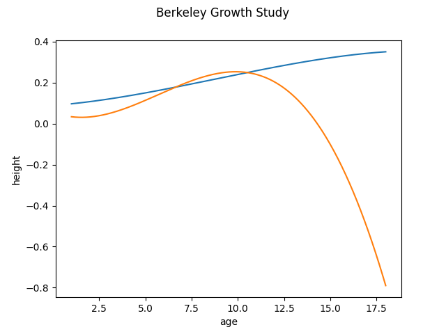
<Figure size 640x480 with 1 Axes>